Year 1 Pure · Chapter 11

Exponential Models

Specification: Edexcel Pure 6 — Exponentials and logarithms · AQA section F

Download chapter PDF Scroll this chapter

In this chapter

1. The number e and y = eˣ
2. The natural logarithm
3. Exponential growth and decay
4. Reduction to linear form
Practice

Key facts — this chapter

$e \approx 2.718$ is the special base where $y = e^x$ has gradient equal to its own height at every point.
$\ln x$ means $\log_e x$ — the inverse of $e^x$ , so $\ln(e^x) = x$ and $e^{\ln x} = x$ .
Growth/decay model: $y = A e^{kt}$ starts at $A$ (when $t = 0$ ); $k > 0$ grows, $k < 0$ decays.
Doubling time is $\dfrac{\ln 2}{k}$ ; half-life is $\dfrac{\ln 2}{|k|}$ .
Reduction to linear form: for $y = ab^x$ , taking logs gives $\log y = (\log b)x + \log a$ — a straight line when $\log y$ is plotted against $x$ .

Lots of real things grow or shrink at a rate proportional to their current size — populations, savings, radioactive decay, cooling drinks. They’re all modelled by the exponential function, and the natural base $e$ is what makes the maths clean.

1. The number e and y = eˣ

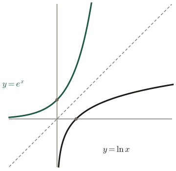
Among all the curves $y = a^x$ , exactly one has the elegant property that its gradient equals its height everywhere. That base is $e \approx 2.718$ .

Key result

For $y = e^x$ , the gradient at any point equals the $y$ -value there:

\frac{dy}{dx} = e^x = y

This is exactly why $e$ shows up whenever a quantity changes at a rate proportional to its current amount.

The curves y = e to the x and y = ln x, reflections of each other in the line y = x — y = eˣ and its inverse y = ln x, mirror images in y = x.

2. The natural logarithm

The inverse of $e^x$ is the natural logarithm $\ln x$ (that is, $\log_e x$ ). It obeys every log law from Chapter 10 — it just has base $e$ .

Key result

\ln(e^x) = x \qquad\text{and}\qquad e^{\ln x} = x

So to undo $e$ , take $\ln$ ; to undo $\ln$ , raise $e$ to the power. This is the key to solving any equation with $e$ or $\ln$ in it.

Worked example 11.1 · Solving with e and ln

Solve $e^{2x} = 7$ , giving your answer to 3 significant figures.

Take $\ln$ of both sides — it cancels the $e$ :
$\ln(e^{2x}) = \ln 7 \;\;\Longrightarrow\;\; 2x = \ln 7$
So
$x = \frac{\ln 7}{2} = 0.973 \;\,(3\text{ s.f.})$

3. Exponential growth and decay

The workhorse model is $y = A e^{kt}$ . Reading off its constants in context is a core exam skill.

Key result

In $y = A e^{kt}$ :

$A$ is the initial value (at $t = 0$ , since $e^0 = 1$ );
$k$ is the growth rate — $k > 0$ grows, $k < 0$ decays;
the doubling time (growth) is $\dfrac{\ln 2}{k}$ , and the half-life (decay) is $\dfrac{\ln 2}{|k|}$ .

Two exponential curves from the same start A: one rising for k greater than 0, one falling for k less than 0 — Same start A; positive k grows, negative k decays.

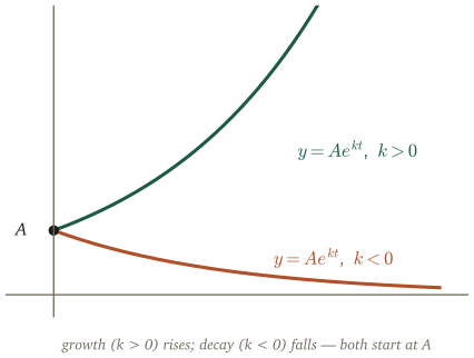
Build a model y = A e^(kt). A sets where it starts; k sets how fast it changes — positive grows, negative decays. The doubling time / half-life updates too.

t runs 0 to 10 · the vertical axis rescales to fit the curve

Worked example 11.2 · A population model

A population is modelled by $P = 8000\,e^{0.05t}$ , where $t$ is in years. (a) Find the population after $12$ years. (b) Find, to the nearest year, when the population reaches $20\,000$ .

(a) Substitute $t = 12$ :
$P = 8000\,e^{0.05 \times 12} = 8000\,e^{0.6} = 14\,600 \;\,(3\text{ s.f.})$
(b) Set $P = 20\,000$ and solve for $t$ :
$8000\,e^{0.05t} = 20\,000 \;\;\Longrightarrow\;\; e^{0.05t} = 2.5$
Take $\ln$ :
$0.05t = \ln 2.5 \;\;\Longrightarrow\;\; t = \frac{\ln 2.5}{0.05} = 18.3\ldots$

So the population reaches $20\,000$ after about $18$ years.

Worked example 11.3 · Half-life of a decay

A radioactive sample has mass $m = 50\,e^{-0.2t}$ grams, with $t$ in days. Find its half-life.

The half-life is when the mass halves, from $50$ to $25$ :
$50\,e^{-0.2t} = 25 \;\;\Longrightarrow\;\; e^{-0.2t} = \tfrac{1}{2}$
Take $\ln$ :
$-0.2t = \ln\tfrac{1}{2} = -\ln 2 \;\;\Longrightarrow\;\; t = \frac{\ln 2}{0.2} = 3.47 \;\text{days} \;\,(3\text{ s.f.})$

Common mistake

The starting amount $A$ is the value at $t = 0$ , not the coefficient of $t$ . In $P = 8000\,e^{0.05t}$ the population starts at $8000$ (because $e^0 = 1$ ), and grows at rate $0.05$ — don’t read $0.05$ as a population.

4. Reduction to linear form

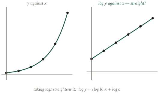
Raw exponential data looks like a curve, which is hard to fit by eye. Taking logs straightens it into a line — and a line you can find the equation of.

Key result

For a model $y = ab^x$ , take logs of both sides:

\log y = \log a + x\log b

Plotting $\log y$ (vertical) against $x$ (horizontal) gives a straight line with gradient $\log b$ and vertical intercept $\log a$ .

Why it works

The relationship $y = ab^x$ is curved, but applying $\log$ turns the product into a sum and brings the power down: $\log(ab^x) = \log a + \log(b^x) = \log a + x\log b$ . That has the form $Y = mX + c$ with $Y = \log y$ , so the transformed data is linear — and a ruler can fit a line where it couldn’t fit a curve.

Left: data on an exponential curve. Right: the same data as a straight line when log y is plotted against x. — log y against x is straight, with gradient log b and intercept log a.

Worked example 11.4 · Finding the model from a straight line

Data fits a model $y = ab^x$ . When $\log_{10} y$ is plotted against $x$ , the line has gradient $0.3$ and vertical intercept $0.6$ . Find $a$ and $b$ .

Compare with $\log y = (\log b)x + \log a$ :
- intercept: $\log_{10} a = 0.6 \;\Longrightarrow\; a = 10^{0.6} = 3.98 \;\,(3\text{ s.f.})$
- gradient: $\log_{10} b = 0.3 \;\Longrightarrow\; b = 10^{0.3} = 2.00 \;\,(3\text{ s.f.})$

So the model is approximately $y = 3.98 \times 2.00^{\,x}$ .

Common mistake

The gradient and intercept give $\log a$ and $\log b$ , not $a$ and $b$ themselves. You must raise the base to those values ( $a = 10^{\text{intercept}}$ , $b = 10^{\text{gradient}}$ ) to recover the constants.

Practice

Twelve questions in three tiers. Try each one properly before opening the solution — the solutions show full method, not just answers. Give non-exact answers to 3 s.f.

Warm-up

1 [3 marks]

Solve, giving exact answers:

$e^x = 5$
$\ln x = 3$

Show solution

(a) Take $\ln$ : $x = \ln 5$ .

(b) Raise $e$ to both sides: $x = e^3$ .

2 [3 marks]

Solve $e^{3x} = 12$ , giving your answer to 3 significant figures.

Show solution

3x = \ln 12 \;\;\Longrightarrow\;\; x = \frac{\ln 12}{3} = 0.828 \;\,(3\text{ s.f.})

3 [2 marks]

The value of a car is modelled by $V = 12000\,e^{-0.15t}$ pounds, $t$ years after purchase. State (a) the purchase value, (b) whether the model is growth or decay.

Show solution

(a) At $t = 0$ : $V = 12000\,e^0 = \pounds 12000$ .

(b) $k = -0.15 < 0$ , so the value decays.

4 [2 marks]

Simplify (a) $\ln(e^4)$ , (b) $e^{\ln 9}$ .

Show solution

(a) $\ln$ and $e$ are inverses: $\ln(e^4) = 4$ .

(b) Likewise $e^{\ln 9} = 9$ .

Standard

5 [4 marks]

A population of bacteria is modelled by $N = 400\,e^{0.08t}$ , where $t$ is in hours.

Find $N$ when $t = 10$ . [2]
Find, to 3 s.f., the time taken for the population to reach $1000$ . [2]

Show solution

(a) $N = 400\,e^{0.8} = 890$ (3 s.f.).

(b) $400\,e^{0.08t} = 1000 \Rightarrow e^{0.08t} = 2.5$ , so

0.08t = \ln 2.5 \;\;\Longrightarrow\;\; t = \frac{\ln 2.5}{0.08} = 11.5 \;\,(3\text{ s.f.})

6 [4 marks]

A cup of coffee cools according to $T = 20 + 60\,e^{-0.04t}$ , where $T$ is in $^\circ$ C and $t$ in minutes.

State the initial temperature. [1]
Find the temperature after $30$ minutes. [1]
Find, to the nearest minute, when the coffee reaches $50^\circ$ C. [2]

Show solution

(a) At $t = 0$ : $T = 20 + 60 = 80^\circ$ C.

(b) $T = 20 + 60\,e^{-1.2} = 38.1^\circ$ C (3 s.f.).

(c) $20 + 60\,e^{-0.04t} = 50 \Rightarrow e^{-0.04t} = \tfrac{30}{60} = \tfrac12$ , so

-0.04t = \ln\tfrac12 = -\ln 2 \;\;\Longrightarrow\;\; t = \frac{\ln 2}{0.04} = 17.3\ldots \approx 17 \text{ min}

7 [4 marks]

A radioactive isotope decays as $m = m_0\,e^{-0.05t}$ ( $t$ in years). Find its half-life, to 3 significant figures.

Show solution

Half-life is when $m = \tfrac12 m_0$ :

e^{-0.05t} = \tfrac12 \;\;\Longrightarrow\;\; -0.05t = -\ln 2 \;\;\Longrightarrow\;\; t = \frac{\ln 2}{0.05} = 13.9 \text{ years}

8 [4 marks]

Data fits the model $y = ab^x$ . When $\log_{10} y$ is plotted against $x$ , a straight line of gradient $0.5$ and vertical intercept $1$ is obtained. Find $a$ and $b$ .

Show solution

Comparing with $\log y = (\log b)x + \log a$ :

$\log_{10} a = 1 \Rightarrow a = 10^1 = 10$ ;
$\log_{10} b = 0.5 \Rightarrow b = 10^{0.5} = 3.16$ (3 s.f.).

Exam style

9 [5 marks]

The mass of a culture is $M = 5\,e^{0.6t}$ grams, $t$ hours after the start.

Find the doubling time, to 3 s.f. [3]
Explain why the doubling time does not depend on the starting mass. [2]

Show solution

(a) Doubling means $M = 2 \times 5 = 10$ :

5\,e^{0.6t} = 10 \Rightarrow e^{0.6t} = 2 \Rightarrow t = \frac{\ln 2}{0.6} = 1.16 \text{ hours}

(b) Setting $M = 2M_0$ gives $e^{kt} = 2$ whatever $M_0$ is — the $M_0$ cancels. So the doubling time $\dfrac{\ln 2}{k}$ depends only on the rate $k$ , not the start.

10 [6 marks]

The temperature of a liquid is modelled by $\theta = 75\,e^{-kt} + 18$ , where $t$ is in minutes. After $5$ minutes the temperature is $60^\circ$ C.

Find the value of $k$ , to 3 s.f. [4]
Find the temperature after $15$ minutes. [2]

Show solution

(a) At $t = 5$ , $\theta = 60$ :

75\,e^{-5k} + 18 = 60 \;\;\Longrightarrow\;\; 75\,e^{-5k} = 42 \;\;\Longrightarrow\;\; e^{-5k} = 0.56

Take $\ln$ : $-5k = \ln 0.56$ , so

k = -\frac{\ln 0.56}{5} = 0.116 \;\,(3\text{ s.f.})

(b) $\theta = 75\,e^{-0.116 \times 15} + 18 = 75\,e^{-1.74} + 18 = 31.2^\circ$ C (3 s.f.).

11 [5 marks]

The table shows values fitting $y = ab^x$ :

$x$	$1$	$2$	$3$
$y$	$12$	$24$	$48$

Explain how the table shows $b = 2$ . [2]
Find $a$ . [3]

Show solution

(a) Each time $x$ increases by $1$ , $y$ multiplies by $2$ ( $12 \to 24 \to 48$ ). For $y = ab^x$ , a unit increase in $x$ multiplies $y$ by $b$ , so $b = 2$ .

(b) Use any data point, say $x = 1$ , $y = 12$ , with $b = 2$ :

12 = a \times 2^1 \;\;\Longrightarrow\;\; a = 6

So $y = 6 \times 2^x$ .

12 [6 marks]

A quantity is modelled by $y = 200\,e^{kt}$ . It is known that $y = 260$ when $t = 4$ .

Find $k$ , to 3 s.f. [3]
Find $y$ when $t = 10$ , to 3 s.f. [2]
Find, to 3 s.f., the value of $t$ for which $y = 500$ . [1]

Show solution

(a) $200\,e^{4k} = 260 \Rightarrow e^{4k} = 1.3$ , so

k = \frac{\ln 1.3}{4} = 0.0656 \;\,(3\text{ s.f.})

(b) $y = 200\,e^{0.0656 \times 10} = 200\,e^{0.656} = 385$ (3 s.f.).

(c) $200\,e^{kt} = 500 \Rightarrow e^{kt} = 2.5$ , so $t = \dfrac{\ln 2.5}{0.0656} = 14.0$ (3 s.f.).