Year 1 Pure · Chapter 13

Applications of Differentiation

Specification: Edexcel Pure 7 — Differentiation · AQA section G

Download chapter PDF Scroll this chapter

In this chapter

1. Tangents and normals
2. Stationary points
3. Maximum or minimum?
4. Optimisation
Practice

Key facts — this chapter

The tangent at a point has gradient $\dfrac{dy}{dx}$ there; the normal is perpendicular, with gradient $-\dfrac{1}{\,dy/dx\,}$ .
A stationary point is where $\dfrac{dy}{dx} = 0$ — the curve is momentarily flat.
Classify with the second derivative: $\dfrac{d^2y}{dx^2} < 0$ is a maximum, $\dfrac{d^2y}{dx^2} > 0$ is a minimum.
A curve is increasing where $\dfrac{dy}{dx} > 0$ and decreasing where $\dfrac{dy}{dx} < 0$ .
Optimisation: write the quantity as a function of one variable, differentiate, set it to $0$ , and solve — then check it’s the max/min you want.

Chapter 12 gave you the derivative; this chapter spends it. Knowing the gradient at every point lets you draw tangents, find a curve’s peaks and troughs, and solve the classic “what’s the biggest/cheapest/fastest?” problems.

1. Tangents and normals

The derivative gives the gradient of the tangent at a point. From there it’s just straight-line geometry (Chapter 4).

Key result

At the point $(x_1, y_1)$ on the curve:

the tangent has gradient $m = \dfrac{dy}{dx}$ there, and equation $y - y_1 = m(x - x_1)$ ;
the normal is perpendicular to it, with gradient $-\dfrac{1}{m}$ .

A curve with a tangent and a normal drawn at a point P, meeting at a right angle — The tangent follows the curve's gradient; the normal crosses it at a right angle.

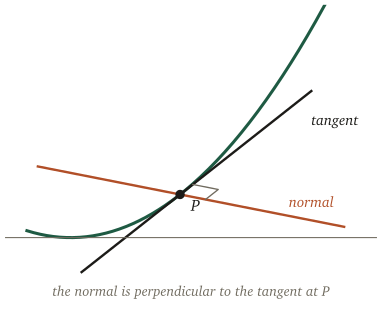
Worked example 13.1 · Tangent and normal at a point

Find the equations of the tangent and normal to $y = x^2 - 3x + 2$ at the point where $x = 3$ .

The point: at $x = 3$ , $y = 9 - 9 + 2 = 2$ , so it’s $(3, 2)$ .
The gradient there: $\dfrac{dy}{dx} = 2x - 3$ , so at $x = 3$ , $m = 3$ .
Tangent (gradient $3$ through $(3,2)$ ):
$y - 2 = 3(x - 3) \;\;\Longrightarrow\;\; y = 3x - 7$
Normal (gradient $-\tfrac{1}{3}$ through $(3,2)$ ):
$y - 2 = -\tfrac{1}{3}(x - 3) \;\;\Longrightarrow\;\; y = -\tfrac{1}{3}x + 3$

2. Stationary points

A stationary point is where the curve flattens out — a maximum, a minimum, or a point of inflection. All of them share one feature: the gradient is zero.

Key result

To find stationary points: solve $\dfrac{dy}{dx} = 0$ . Each solution is the $x$ -coordinate of a stationary point; substitute back into $y$ for its height.

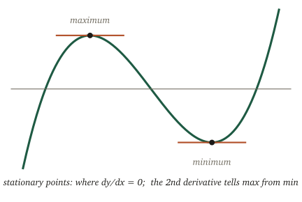
A cubic curve with a local maximum and a local minimum, each with a flat tangent — At a maximum and a minimum alike, the tangent is flat — dy/dx = 0.

Worked example 13.2 · Finding the stationary points

Find the coordinates of the stationary points of $y = x^3 - 3x$ .

Differentiate and set to zero:
$\frac{dy}{dx} = 3x^2 - 3 = 0 \;\;\Longrightarrow\;\; x^2 = 1 \;\;\Longrightarrow\;\; x = \pm 1$
Find the $y$ -values: $x = 1 \Rightarrow y = -2$ ; $x = -1 \Rightarrow y = 2$ .

So the stationary points are $(1, -2)$ and $(-1, 2)$ .

3. Maximum or minimum?

Finding a stationary point is half the job; you also need to know which kind. The fastest test is the second derivative.

Key result

At a stationary point, look at $\dfrac{d^2y}{dx^2}$ :

$\dfrac{d^2y}{dx^2} < 0$ — a maximum (gradient is decreasing through it: the curve is bending down);
$\dfrac{d^2y}{dx^2} > 0$ — a minimum (gradient increasing: bending up).

(If it’s zero, the test is inconclusive — check the gradient either side instead.)

Worked example 13.3 · Classifying the stationary points

Classify the stationary points of $y = x^3 - 3x$ from Example 13.2.

The second derivative:
$\frac{d^2y}{dx^2} = 6x$
Test each point:
- at $x = -1$ : $\dfrac{d^2y}{dx^2} = -6 < 0$ , so $(-1, 2)$ is a maximum;
- at $x = 1$ : $\dfrac{d^2y}{dx^2} = 6 > 0$ , so $(1, -2)$ is a minimum.

Common mistake

Substitute the stationary point’s $x$ into the second derivative, not the first (which is zero there by definition, so tells you nothing). And the sign is what matters — a negative second derivative means a maximum, which catches people out.

4. Optimisation

The big payoff: real problems asking for the largest area, smallest cost, maximum volume. The plan is always the same — get the quantity as a function of one variable, then differentiate to find the turning point.

The optimisation routine

Write the quantity to optimise as a function of one variable (use any given constraint to eliminate the others).
Differentiate and set $\dfrac{dy}{dx} = 0$ ; solve for the variable.
Check it’s the max (or min) you want — the second derivative, or context.
Answer the question actually asked (often the optimal value, not just where).

Cut a square of side x from each corner of a 12 × 12 sheet and fold up the sides. Vary x and watch the volume V = x(12 − 2x)² — it peaks where dV/dx = 0.

the dot is your current x · the curve peaks at x = 2, V = 128 cm³

Worked example 13.4 · The largest open box

An open box is made from a $12\text{ cm} \times 12\text{ cm}$ square of card by cutting a square of side $x$ from each corner and folding up the sides. Find the value of $x$ that maximises the volume, and the maximum volume.

After cutting and folding, the base is $(12 - 2x)$ by $(12 - 2x)$ and the height is $x$ , so
$V = x(12 - 2x)^2$
Expand and differentiate:
$V = 144x - 48x^2 + 4x^3 \;\;\Longrightarrow\;\; \frac{dV}{dx} = 144 - 96x + 12x^2$
Set $\dfrac{dV}{dx} = 0$ :
$\begin{aligned} 12x^2 - 96x + 144 &= 0 \\[0.3em] x^2 - 8x + 12 &= 0 \\[0.3em] (x - 2)(x - 6) &= 0 \end{aligned}$
So $x = 2$ or $x = 6$ . But $x = 6$ leaves no base ( $12 - 2x = 0$ ), so $x = 2$ .
Confirm it’s a maximum: $\dfrac{d^2V}{dx^2} = -96 + 24x$ , which at $x = 2$ is $-48 < 0$ — a maximum. ✓

The maximum volume is $V = 2(12 - 4)^2 = 2 \times 64 = 128 \text{ cm}^3$ .

Common mistake

Don’t stop at $\dfrac{dV}{dx} = 0$ . Always discard solutions that don’t make physical sense (here $x = 6$ gives a flat box), confirm you’ve found a maximum, and read the question — it usually wants the maximum volume, not just the $x$ .

Practice

Twelve questions in three tiers. Try each one properly before opening the solution — the solutions show full method, not just answers.

Warm-up

1 [3 marks]

Find the equation of the tangent to $y = x^2 + 1$ at the point $(2, 5)$ .

Show solution

$\dfrac{dy}{dx} = 2x$ , so at $x = 2$ the gradient is $4$ . Tangent through $(2, 5)$ :

y - 5 = 4(x - 2) \;\;\Longrightarrow\;\; y = 4x - 3

2 [3 marks]

Find the $x$ -coordinates of the stationary points of $y = x^2 - 6x + 5$ .

Show solution

$\dfrac{dy}{dx} = 2x - 6 = 0 \Rightarrow x = 3$ . (One stationary point, at $x = 3$ .)

3 [3 marks]

A curve has $\dfrac{dy}{dx} = 3x^2 - 12$ . State whether it is increasing or decreasing at (a) $x = 1$ , (b) $x = 3$ .

Show solution

(a) At $x = 1$ : $3 - 12 = -9 < 0$ , so decreasing.

(b) At $x = 3$ : $27 - 12 = 15 > 0$ , so increasing.

4 [3 marks]

The curve $y = x^2 - 4x$ has a stationary point. Find its coordinates and use the second derivative to state its nature.

Show solution

$\dfrac{dy}{dx} = 2x - 4 = 0 \Rightarrow x = 2$ , $y = 4 - 8 = -4$ . Point $(2, -4)$ .

$\dfrac{d^2y}{dx^2} = 2 > 0$ , so it is a minimum.

Standard

5 [4 marks]

Find the equation of the normal to $y = x^2 - 5x + 6$ at the point where $x = 1$ .

Show solution

At $x = 1$ : $y = 1 - 5 + 6 = 2$ , so the point is $(1, 2)$ .
$\dfrac{dy}{dx} = 2x - 5$ , so the tangent gradient at $x = 1$ is $-3$ ; the normal gradient is $\tfrac{1}{3}$ .
Normal through $(1, 2)$ :
$y - 2 = \tfrac{1}{3}(x - 1) \;\;\Longrightarrow\;\; y = \tfrac{1}{3}x + \tfrac{5}{3}$

6 [5 marks]

Find and classify the stationary points of $y = 2x^3 - 3x^2 - 12x$ .

Show solution

$\dfrac{dy}{dx} = 6x^2 - 6x - 12 = 0 \Rightarrow x^2 - x - 2 = 0 \Rightarrow (x-2)(x+1) = 0$ , so $x = 2$ or $x = -1$ .
Heights: $x = 2 \Rightarrow y = 16 - 12 - 24 = -20$ ; $x = -1 \Rightarrow y = -2 - 3 + 12 = 7$ .
Classify with $\dfrac{d^2y}{dx^2} = 12x - 6$ :
- at $x = -1$ : $-18 < 0$ , so $(-1, 7)$ is a maximum;
- at $x = 2$ : $18 > 0$ , so $(2, -20)$ is a minimum.

7 [4 marks]

The curve $y = x^3 - 12x + 3$ has a tangent that is parallel to the $x$ -axis. Find the coordinates of the points where this happens.

Show solution

A tangent parallel to the $x$ -axis has gradient $0$ :

\frac{dy}{dx} = 3x^2 - 12 = 0 \;\;\Longrightarrow\;\; x = \pm 2

Heights: $x = 2 \Rightarrow y = 8 - 24 + 3 = -13$ ; $x = -2 \Rightarrow y = -8 + 24 + 3 = 19$ .

Points: $(2, -13)$ and $(-2, 19)$ .

8 [5 marks]

A farmer has $40$ m of fencing to enclose a rectangular pen against a wall (so only three sides are fenced). If the side perpendicular to the wall is $x$ m, the area is $A = x(40 - 2x)$ .

Find the value of $x$ that maximises the area. [3]
Find the maximum area. [2]

Show solution

(a) Expand and differentiate:

A = 40x - 2x^2 \;\;\Longrightarrow\;\; \frac{dA}{dx} = 40 - 4x = 0 \;\;\Longrightarrow\;\; x = 10

( $\dfrac{d^2A}{dx^2} = -4 < 0$ , confirming a maximum.)

(b) $A = 10(40 - 20) = 10 \times 20 = 200 \text{ m}^2$ .

9 [4 marks]

Show that the curve $y = x^3 + 3x^2 + 5x - 2$ has no stationary points.

Show solution

$\dfrac{dy}{dx} = 3x^2 + 6x + 5$ . Stationary points need this to be zero, so check its discriminant:

\Delta = 6^2 - 4(3)(5) = 36 - 60 = -24 < 0

The quadratic has no real roots, so $\dfrac{dy}{dx}$ is never zero — there are no stationary points. (Indeed $\dfrac{dy}{dx} > 0$ everywhere, so the curve is always increasing.) ∎

Exam style

10 [6 marks]

The curve $C$ has equation $y = x^3 - 6x^2 + 9x + 1$ .

Find the coordinates of the two stationary points of $C$ . [3]
Determine the nature of each. [2]
Find the equation of the tangent to $C$ at $x = 0$ . [1]

Show solution

(a) $\dfrac{dy}{dx} = 3x^2 - 12x + 9 = 0 \Rightarrow x^2 - 4x + 3 = 0 \Rightarrow (x-1)(x-3) = 0$ . At $x = 1$ : $y = 1 - 6 + 9 + 1 = 5$ . At $x = 3$ : $y = 27 - 54 + 27 + 1 = 1$ . Points: $(1, 5)$ and $(3, 1)$ .

(b) $\dfrac{d^2y}{dx^2} = 6x - 12$ : at $x = 1$ , $-6 < 0$ (maximum); at $x = 3$ , $6 > 0$ (minimum).

(c) At $x = 0$ : $y = 1$ and the gradient is $9$ . Tangent: $y = 9x + 1$ .

11 [6 marks]

A closed cylinder has radius $r$ and a fixed volume. Its surface area is modelled by $S = 2\pi r^2 + \dfrac{600}{r}$ (in cm²).

Find $\dfrac{dS}{dr}$ . [2]
Find the value of $r$ that minimises the surface area, to 3 s.f. [3]
Verify it is a minimum. [1]

Show solution

(a) Write $S = 2\pi r^2 + 600r^{-1}$ :

\frac{dS}{dr} = 4\pi r - 600r^{-2} = 4\pi r - \frac{600}{r^2}

(b) Set $\dfrac{dS}{dr} = 0$ :

4\pi r = \frac{600}{r^2} \;\;\Longrightarrow\;\; r^3 = \frac{600}{4\pi} = \frac{150}{\pi} \;\;\Longrightarrow\;\; r = 3.63 \;\,(3\text{ s.f.})

(c) $\dfrac{d^2S}{dr^2} = 4\pi + \dfrac{1200}{r^3} > 0$ for $r > 0$ , so it is a minimum. ✓

12 [6 marks]

A rectangle has its base on the $x$ -axis and its top two corners on the curve $y = 12 - x^2$ (with $x > 0$ on the right). The corners are at $(\pm x, 0)$ and $(\pm x, 12 - x^2)$ , so its area is $A = 2x(12 - x^2)$ .

Find the value of $x$ that maximises the area. [4]
Find the maximum area. [2]

Show solution

(a) Expand and differentiate:

A = 24x - 2x^3 \;\;\Longrightarrow\;\; \frac{dA}{dx} = 24 - 6x^2 = 0

x^2 = 4 \;\;\Longrightarrow\;\; x = 2 \quad (x > 0)

(taking $x > 0$ ; $\dfrac{d^2A}{dx^2} = -12x < 0$ confirms a maximum).

(b) $A = 2(2)(12 - 4) = 4 \times 8 = 32$ .