Year 2 Statistics · Chapter 1

Regression and Correlation

Specification: Edexcel Paper 3 §2.2, 5.1 — Correlation and regression · AQA section L2, O1

Download chapter PDF Scroll this chapter

In this chapter

1. The product moment correlation coefficient
2. Testing for correlation
3. Straightening curves
Practice

Key facts — this chapter

The product moment correlation coefficient $r$ measures the strength of linear correlation in a sample. Always $-1 \le r \le 1$ : $r = 1$ is perfect positive linear correlation, $r = -1$ perfect negative, and $r = 0$ no linear correlation.
Find $r$ with a calculator. It has no units, and it is unchanged by coding either variable with a positive scale factor.
To test for correlation in the population, use its correlation coefficient $\rho$ : $H_0: \rho = 0$ against $H_1: \rho > 0$ or $\rho < 0$ (one-tailed) or $\rho \ne 0$ (two-tailed).
Compare $r$ with the critical value for the sample size and significance level. If $r$ is beyond it, in the direction of $H_1$ , reject $H_0$ . With a p-value, reject when the p-value is at most the significance level.
A model $y = ax^n$ becomes the straight line $\log y = \log a + n\log x$ . A model $y = kb^x$ becomes $\log y = \log k + x\log b$ .

Year 1 described correlation in words and used a regression line to make predictions. This chapter puts a number on the strength of a linear relationship, then asks the question a statistician must: is the pattern in this sample strong enough to believe it holds in the whole population? It ends by straightening curves, so that the tools of linear regression can fit exponential and power models too.

1. The product moment correlation coefficient

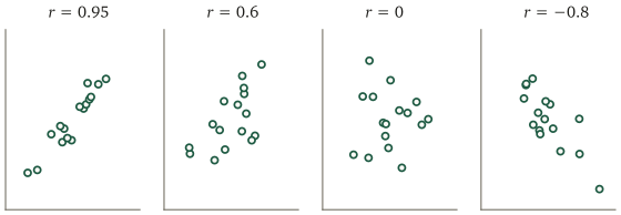
The closer the points lie to a straight line, the closer r is to 1 or −1. Its sign gives the direction.

Reading the coefficient

$r$ close to $1$ : strong positive linear correlation.
$r$ close to $-1$ : strong negative linear correlation.
$r$ close to $0$ : little or no linear correlation.

Why it works

$r = \dfrac{S_{xy}}{\sqrt{S_{xx}S_{yy}}}$ , where $S_{xy} = \sum(x - \bar x)(y - \bar y)$ measures how $x$ and $y$ vary together, and $S_{xx}$ and $S_{yy}$ measure how each varies on its own. Points above and to the right of $(\bar x, \bar y)$ , or below and to the left, make $S_{xy}$ positive; the division scales the result to lie between $-1$ and $1$ .

Common mistake

$r$ measures linear correlation only. Points lying on a U-shaped curve can give $r$ near $0$ , even though $y$ depends strongly on $x$ . Always look at the scatter diagram before trusting $r$ .

Worked example 1.1 · Finding the coefficient

A kiosk records the hours of sunshine, $x$ , and the number of ice creams sold, $y$ , on eight days. Find the product moment correlation coefficient and interpret it.

$x$ (hours)	2	3	4	5	6	7	8	9
$y$ (sales)	31	45	38	52	49	63	56	70

Sunshine and ice cream sales

The calculator’s two-variable statistics mode gives $r = 0.915$ (3 s.f.).

In context

There is strong positive linear correlation between hours of sunshine and ice cream sales: sunnier days tend to bring more sales.

On your calculator

Enter the data in the two-variable statistics or linear regression mode, with $x$ and $y$ in separate columns. The results list $r$ alongside the coefficients $a$ and $b$ of the regression line $y = a + bx$ .

2. Testing for correlation

A sample of eight days gives $r = 0.915$ . Would a different eight days give something similar, or could the pattern be chance? A hypothesis test decides, using the population correlation coefficient $\rho$ (the Greek letter rho).

Testing for correlation

State $H_0: \rho = 0$ (no correlation in the population).
State $H_1$ : $\rho > 0$ or $\rho < 0$ if a direction is suggested (one-tailed), or $\rho \ne 0$ if not (two-tailed).
Find the critical value for the sample size $n$ and the significance level. For a two-tailed test, use half the significance level in each tail.
Reject $H_0$ if $r$ is beyond the critical value in the direction of $H_1$ , and conclude in context.

The critical values come from a table in the formula booklet; questions state the ones you need. The table assumes the data come from a bivariate Normal distribution, so that both variables are roughly Normal.

Worked example 1.2 · A one-tailed test

Using the data in Example 1.1, test at the 1% level whether there is positive correlation between hours of sunshine and ice cream sales. The critical value for $n = 8$ at 1% (one-tailed) is $0.7887$ .

$H_0: \rho = 0$ and $H_1: \rho > 0$ , where $\rho$ is the population correlation coefficient.
$r = 0.915$ , which is more than $0.7887$ , so the result is significant: reject $H_0$ .

In context

There is sufficient evidence at the 1% level of positive correlation between hours of sunshine and ice cream sales.

Common mistake

Hypotheses are about the population, so they use $\rho$ , never $r$ . Writing $H_0: r = 0$ loses the mark: $r$ is a number you calculate, and it certainly isn’t exactly $0$ .

Worked example 1.3 · A two-tailed test

A teacher suspects that the time students spend on social media is related to their sleep, but has no view on the direction. For a sample of 12 students, $r = -0.54$ . Test at the 5% level whether there is correlation. The critical value for $n = 12$ at 2.5% (one-tailed) is $0.5760$ .

$H_0: \rho = 0$ and $H_1: \rho \ne 0$ .
Two-tailed at 5% means 2.5% in each tail, so the critical values are $\pm 0.5760$ .
$-0.54$ lies between $-0.5760$ and $0.5760$ : not significant, so do not reject $H_0$ .

In context

There is insufficient evidence at the 5% level of correlation between time on social media and sleep.

Drag the points, or add and remove them. The product moment correlation coefficient r moves along the scale underneath, where the shaded part is the critical region for the test you choose. When r lands in it, the sample is evidence of correlation in the population.

Software often reports a p-value instead: the probability, if $\rho = 0$ , of a sample correlation at least as extreme as the one observed.

Worked example 1.4 · Using a p-value

A researcher records the daily step count and the hours of sleep of a random sample of 25 adults, and tests $H_0: \rho = 0$ against $H_1: \rho > 0$ . The sample gives $r = 0.43$ , with a p-value of $0.016$ . State the conclusion at the 1% level, and at the 5% level.

At 1%: $0.016 > 0.01$ , so the result is not significant: do not reject $H_0$ .
At 5%: $0.016 < 0.05$ , so the result is significant: reject $H_0$ .

In context

At the 1% level there is insufficient evidence of positive correlation between step count and sleep; at the 5% level there is sufficient evidence. The stricter the test, the stronger the evidence it demands.

Common mistake

Not rejecting $H_0$ does not prove that $\rho = 0$ . It means this sample isn’t strong enough evidence against it. And rejecting $H_0$ shows correlation, not causation.

3. Straightening curves

Many relationships are curved: populations grow exponentially, and areas and masses grow as powers of length. Taking logarithms turns both kinds of curve into straight lines, as in Chapter 11 of Year 1 Pure, and a straight line is something regression can fit.

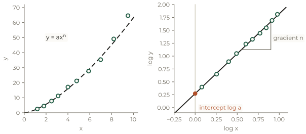
Changing the variables

\begin{aligned} y = ax^n \;&\Rightarrow\; \log y = \log a + n\log x \\ y = kb^x \;&\Rightarrow\; \log y = \log k + (\log b)x \end{aligned}

For $y = ax^n$ , plot $\log y$ against $\log x$ : the gradient is $n$ and the intercept $\log a$ . For $y = kb^x$ , plot $\log y$ against $x$ : the gradient is $\log b$ and the intercept $\log k$ .

Data from y = axⁿ lie on a curve; plotted as log y against log x, they lie close to a line with gradient n.

Worked example 1.5 · A power model

A student times a pendulum of length $l$ metres and finds its period $T$ seconds for several lengths. She models $T = al^n$ . The regression line of $\log_{10} T$ on $\log_{10} l$ is $\log_{10} T = 0.303 + 0.498\log_{10} l$ . Find $a$ and $n$ , and estimate the period of a pendulum $0.8$ m long.

Compare with $\log T = \log a + n\log l$ : $n = 0.498$ and $\log_{10} a = 0.303$ , so $a = 10^{0.303} = 2.01$ (3 s.f.).
The model is $T = 2.01\,l^{0.498}$ , so for $l = 0.8$ , $T = 2.009\ldots \times 0.8^{0.498} = 1.80$ s (3 s.f.).

In context

$T \approx 2.01\,l^{0.5}$ : the period grows with the square root of the length, as physics predicts.

Worked example 1.6 · An exponential model

The number of bacteria $N$ in a culture is counted at times $t$ hours and modelled by $N = kb^t$ . The regression line of $\log_{10} N$ on $t$ is $\log_{10} N = 2.1 + 0.035t$ . Find $k$ and $b$ , interpret them, and estimate $N$ when $t = 10$ .

Compare with $\log N = \log k + (\log b)t$ : $\log_{10} k = 2.1$ and $\log_{10} b = 0.035$ .
So $k = 10^{2.1} = 126$ (3 s.f.) and $b = 10^{0.035} = 1.08$ (3 s.f.).
At $t = 10$ : $\log_{10} N = 2.1 + 0.35 = 2.45$ , so $N = 10^{2.45} = 282$ (3 s.f.).

In context

The culture starts with about 126 bacteria, and the number grows by about 8.4% each hour, since $b = 1.0839\ldots$ . After 10 hours the model predicts about 282 bacteria.

Common mistake

Keep the logarithm in the intercept. The intercept of the straight line is $\log k$ , not $k$ , so $k = 10^{\text{intercept}}$ . And a model only describes the range of the data it was fitted to: estimates far outside it are extrapolation.

Practice

Twelve questions in three tiers. Try each one properly before opening the solution. The solutions show the full method, not just answers. Critical values are given in each question; logarithms are to base 10 unless a question says otherwise. Give answers to 3 significant figures where they aren’t exact.

Warm-up

1 [3 marks]

Describe the correlation shown by each value of the product moment correlation coefficient: (a) $r = 0.87$ , (b) $r = -0.12$ , (c) $r = -0.95$ .

Show solution

(a) Strong positive linear correlation. (b) Very weak negative linear correlation: essentially none. (c) Strong negative linear correlation.

2 [4 marks]

A biologist believes that taller people have longer arm spans. For a sample of 8 adults, $r = 0.71$ . Test her belief at the 5% level. The critical value for $n = 8$ at 5% (one-tailed) is $0.6215$ .

Show solution

$H_0: \rho = 0$ and $H_1: \rho > 0$ , where $\rho$ is the population correlation coefficient.

$0.71 > 0.6215$ , so the result is significant: reject $H_0$ . There is sufficient evidence at the 5% level of positive correlation between height and arm span.

3 [4 marks]

For a sample of 20 cars, the correlation between engine size and the number of faults reported is $r = 0.41$ . Test at the 5% level whether there is correlation. The critical value for $n = 20$ at 2.5% (one-tailed) is $0.4438$ .

Show solution

$H_0: \rho = 0$ and $H_1: \rho \ne 0$ . Two-tailed at 5%, so compare with $\pm 0.4438$ .

$0.41 < 0.4438$ , so the result is not significant: do not reject $H_0$ . There is insufficient evidence at the 5% level of correlation between engine size and faults.

4 [4 marks]

Write each model as a straight line, stating what to plot and the gradient and intercept: (a) $y = 3x^2$ , (b) $y = 5 \times 2^x$ .

Show solution

(a) $\log y = \log 3 + 2\log x$ : plot $\log y$ against $\log x$ . The gradient is $2$ and the intercept $\log 3 = 0.477$ .

(b) $\log y = \log 5 + (\log 2)x$ : plot $\log y$ against $x$ . The gradient is $\log 2 = 0.301$ and the intercept $\log 5 = 0.699$ .

Standard

5 [6 marks]

A coach records the hours of training, $x$ , and a performance score, $y$ , for six athletes in one month.

$x$ (hours)	12	15	17	20	24	28
$y$ (score)	56	54	66	61	71	66

Find the product moment correlation coefficient. [1]
Test at the 5% level whether more training goes with a higher score. The critical value for $n = 6$ at 5% (one-tailed) is $0.7293$ . [4]
The critical value at 2.5% (one-tailed) is $0.8114$ . Would the conclusion be the same at the 2.5% level? [1]

Show solution

(a) From a calculator, $r = 0.751$ (3 s.f.).

(b) $H_0: \rho = 0$ and $H_1: \rho > 0$ . $0.751 > 0.7293$ , so reject $H_0$ : there is sufficient evidence at the 5% level of positive correlation between training hours and score.

(c) No: $0.751 < 0.8114$ , so at 2.5% the result would not be significant.

6 [4 marks]

A quantity is modelled by $y = ax^n$ . The regression line of $\log y$ on $\log x$ is $\log y = 0.3 + 0.8\log x$ . Find $a$ and $n$ , and estimate $y$ when $x = 20$ .

Show solution

$n = 0.8$ and $\log a = 0.3$ , so $a = 10^{0.3} = 2.00$ (3 s.f.).

At $x = 20$ : $y = 1.995\ldots \times 20^{0.8} = 21.9$ .

7 [5 marks]

The value $V$ pounds of a car $t$ years after it was new is modelled by $V = kb^t$ . The regression line of $\log V$ on $t$ is $\log V = 4.2 - 0.06t$ . Find $k$ and $b$ , and interpret each in context.

Show solution

$\log k = 4.2$ , so $k = 10^{4.2} = 15\,800$ (3 s.f.): the model’s value of the car when new, about £15,800.

$\log b = -0.06$ , so $b = 10^{-0.06} = 0.871$ (3 s.f.): each year the car keeps about 87.1% of its value, losing about 12.9% a year.

8 [3 marks]

A test of $H_0: \rho = 0$ against $H_1: \rho < 0$ gives a p-value of $0.018$ . State, with a reason, the conclusion at the 1% level and at the 5% level.

Show solution

At 1%: $0.018 > 0.01$ , so do not reject $H_0$ : insufficient evidence of negative correlation.

At 5%: $0.018 < 0.05$ , so reject $H_0$ : sufficient evidence of negative correlation.

9 [4 marks]

A scatter diagram shows points lying close to a U-shaped curve, but $r = 0.02$ . Explain how both can be true. [2]
After a test finds insufficient evidence of correlation, a researcher writes “this proves the two variables are not related”. Give two criticisms. [2]

Show solution

(a) $r$ measures linear correlation only. On a U-shape, $y$ falls then rises, so the linear trends cancel and $r$ is near $0$ , even though $y$ depends strongly on $x$ .

(b) Not rejecting $H_0$ is not proof that $\rho = 0$ : the sample may just be too small to show the correlation. And the test looks only for linear correlation, so the variables could still be related in a non-linear way.

Exam style

10 [9 marks]

A café owner records the midday temperature, $x$ °C, and the number of hot drinks sold, $y$ , on eight days.

$x$ (°C)	4	7	9	12	14	17	19	22
$y$ (drinks)	82	85	74	79	64	71	60	66

Find the product moment correlation coefficient. [1]
Test at the 5% level whether there is correlation between temperature and hot drink sales. The critical value for $n = 8$ at 2.5% (one-tailed) is $0.7067$ . [4]
The critical value for $n = 8$ at 0.5% (one-tailed) is $0.8343$ . State the conclusion of the same test at the 1% level. [2]
State an assumption needed for the test to be valid. [2]

Show solution

(a) From a calculator, $r = -0.826$ (3 s.f.).

(b) $H_0: \rho = 0$ and $H_1: \rho \ne 0$ . Two-tailed at 5%, so compare with $\pm 0.7067$ . $-0.826 < -0.7067$ , so reject $H_0$ : there is sufficient evidence at the 5% level of correlation between temperature and hot drink sales.

(c) At 1% two-tailed the critical values are $\pm 0.8343$ , and $-0.826$ lies between them: do not reject $H_0$ . There is insufficient evidence at the 1% level.

(d) The data come from a bivariate Normal distribution: temperature and sales are each roughly Normally distributed. (The eight days should also be a random sample.)

11 [8 marks]

A fisheries officer models the mass $m$ grams of a species of fish by $m = al^n$ , where $l$ cm is its length. From fish between 10 cm and 40 cm long, the regression line of $\log m$ on $\log l$ is $\log m = -1.9 + 3.05\log l$ .

Find $a$ and $n$ . [3]
Estimate the mass of a fish 30 cm long. [2]
Explain why $n$ close to $3$ is reasonable. [1]
Comment on using the model for a fish 80 cm long. [2]

Show solution

(a) $n = 3.05$ and $\log a = -1.9$ , so $a = 10^{-1.9} = 0.0126$ (3 s.f.).

(b) $\log m = -1.9 + 3.05\log 30 = 2.605\ldots$ , so $m = 10^{2.605\ldots} = 403$ g.

(c) Mass is proportional to volume, and a fish that is twice as long is roughly twice as wide and twice as deep: the volume grows as the cube of the length.

(d) 80 cm is far outside the 10–40 cm range of the data, so this is extrapolation and the estimate is unreliable.

12 [6 marks]

A variable is modelled by $y = kb^x$ . Using natural logarithms, the regression line of $\ln y$ on $x$ is $\ln y = 1.2 + 0.4x$ .

Find $k$ and $b$ . [3]
Estimate $y$ when $x = 5$ . [2]
Write the model in the form $y = ke^{cx}$ . [1]

Show solution

(a) $\ln k = 1.2$ , so $k = e^{1.2} = 3.32$ (3 s.f.). $\ln b = 0.4$ , so $b = e^{0.4} = 1.49$ (3 s.f.).

(b) $\ln y = 1.2 + 2 = 3.2$ , so $y = e^{3.2} = 24.5$ .

(c) $y = e^{1.2 + 0.4x} = 3.32e^{0.4x}$ .