Year 2 Statistics · Chapter 4

Normal Hypothesis Tests

Specification: Edexcel Paper 3 §5.3 — Testing the mean of a Normal distribution · AQA section O3

Download chapter PDF Scroll this chapter

In this chapter

1. The distribution of the sample mean
2. Testing the mean
3. Critical regions
4. Two-tailed tests
5. Choosing the sample size
Practice

Key facts — this chapter

If $X \sim N(\mu, \sigma^2)$ , the mean of a random sample of $n$ observations has $\bar X \sim N\!\left(\mu, \dfrac{\sigma^2}{n}\right)$ : the same centre, with standard deviation $\dfrac{\sigma}{\sqrt n}$ .
To test a claim about the mean: $H_0: \mu = \mu_0$ against $H_1: \mu > \mu_0$ or $\mu < \mu_0$ (one-tailed) or $\mu \ne \mu_0$ (two-tailed).
Assuming $H_0$ , $\bar X \sim N\!\left(\mu_0, \dfrac{\sigma^2}{n}\right)$ . The p-value is the probability of a sample mean at least as extreme as the one observed. Reject $H_0$ if it is at most the significance level, or half of it in each tail of a two-tailed test.
Equivalently, find the critical value of $\bar x$ , or compare $z = \dfrac{\bar x - \mu_0}{\sigma / \sqrt n}$ with the critical value of $Z$ .
The test needs a random sample and a known, given or assumed standard deviation. Conclude in context, and never claim $H_0$ is proved.

Year 1 tested claims about a proportion using the binomial distribution. Most claims in science and industry are about a mean instead: the average mass of a loaf, the average life of a battery. One measurement proves little, because individuals vary. The mean of a sample varies much less, and that is what makes it a useful test statistic.

1. The distribution of the sample mean

The sample mean

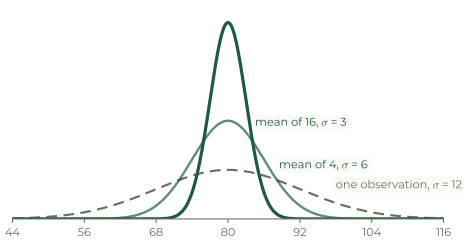
If $X \sim N(\mu, \sigma^2)$ and $\bar X$ is the mean of a random sample of $n$ observations of $X$ , then

\bar X \sim N\!\left(\mu, \frac{\sigma^2}{n}\right)

Three Normal curves centred on 80. The widest, dashed, is a single observation X with standard deviation 12. A taller, narrower curve is the mean of 4 observations, standard deviation 6, and the tallest and narrowest is the mean of 16 observations, standard deviation 3 — Averaging cancels out much of the variation: the mean of 16 observations has a quarter of the standard deviation of one.

Why it works

A sample mean of $n$ values is typically closer to $\mu$ than a single value, because high and low values tend to cancel. The variance falls by a factor of $n$ , so the standard deviation falls by a factor of $\sqrt n$ : four times the sample gives half the spread.

Worked example 4.1 · The mean of a sample

$X \sim N(80, 12^2)$ . A random sample of 16 observations is taken. Find the probability that the sample mean exceeds $85$ .

$\bar X \sim N\!\left(80, \dfrac{12^2}{16}\right) = N(80, 3^2)$ .
$P(\bar X > 85) = 0.0478$ (4 d.p.).

In context

A single observation exceeds 85 about a third of the time, but the mean of 16 does so less than 5% of the time.

Common mistake

Divide the variance by $n$ , not the standard deviation. $\bar X$ has variance $\dfrac{144}{16} = 9$ and standard deviation $3$ , not $\dfrac{12}{16}$ .

2. Testing the mean

Testing a claim about the mean

State $H_0: \mu = \mu_0$ and $H_1$ , with $\mu$ the population mean.
Assuming $H_0$ , $\bar X \sim N\!\left(\mu_0, \dfrac{\sigma^2}{n}\right)$ .
Find the p-value: the probability of a sample mean at least as extreme as $\bar x$ , in the direction of $H_1$ .
Compare it with the significance level, and conclude in context.

Worked example 4.2 · Has the mean fallen?

The masses of loaves from a bakery are Normally distributed with mean $800$ g and standard deviation $15$ g. After a machine is replaced, a random sample of 25 loaves has mean mass $794$ g. Assuming the standard deviation is unchanged, test at the 5% level whether the mean mass has decreased.

$H_0: \mu = 800$ and $H_1: \mu < 800$ , where $\mu$ is the mean mass in grams.
Assuming $H_0$ , $\bar X \sim N\!\left(800, \dfrac{15^2}{25}\right) = N(800, 3^2)$ .
The p-value is $P(\bar X \le 794) = 0.0228$ (4 d.p.). Standardised, $794$ is $z = \dfrac{794 - 800}{3} = -2$ .
$0.0228 < 0.05$ , so the result is significant: reject $H_0$ .

In context

There is sufficient evidence at the 5% level that the mean mass of the loaves has decreased.

Common mistake

The test uses the distribution of the mean, $N(800, 3^2)$ , not the distribution of one loaf, $N(800, 15^2)$ . With the wrong one, $794$ looks ordinary: it is only $0.4$ standard deviations below $800$ for a single loaf.

3. Critical regions

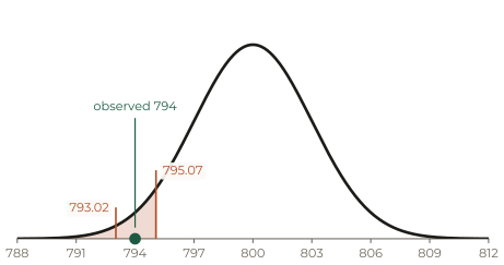
The critical region is the set of sample means that would lead to rejecting $H_0$ , and its boundary is the critical value. For a continuous distribution the region has probability exactly equal to the significance level.

The Normal curve for the sample mean, centred on 800 with standard deviation 3. The lower tail below 795.07 is shaded as the 5% critical region; below that, the 1% critical value 793.02 is marked. The observed mean, 794, lies inside the 5% region but outside the 1% region — Examples 4.2 and 4.3: 794 is in the 5% critical region but not in the 1% one.

Worked example 4.3 · A stricter test

For the test in Example 4.2, find the critical region at the 1% level, and state the conclusion at that level.

$P(Z < z) = 0.01$ gives $z = -2.3263$ , so the critical value, to 2 d.p., is
$800 - 2.3263 \times 3 = 793.02$
and the critical region is $\bar X < 793.02$ .
$794$ is not in the critical region: do not reject $H_0$ .

In context

At the 1% level there is insufficient evidence that the mean mass has decreased. The same sample is significant at 5% but not at 1%.

A population is Normal with mean 50 and standard deviation 10 (dashed). The solid curve is the distribution of the mean of a sample of n: add to the sample and watch it narrow. The shaded tail is the critical region for testing H₀: μ = 50; move the observed sample mean and see whether it lands inside.

4. Two-tailed tests

When the question asks whether the mean has changed, without a direction, the test is two-tailed: split the significance level equally between the two tails.

Worked example 4.4 · Has the mean changed?

A machine cuts rods whose lengths are Normally distributed with standard deviation $0.4$ cm. It should cut them to a mean length of $10$ cm. A random sample of 20 rods has mean length $10.18$ cm. Test at the 5% level whether the mean length has changed.

$H_0: \mu = 10$ and $H_1: \mu \ne 10$ .
Assuming $H_0$ , $\bar X \sim N\!\left(10, \dfrac{0.4^2}{20}\right)$ , with standard deviation $\dfrac{0.4}{\sqrt{20}} = 0.0894\ldots$
$10.18$ is above $10$ , so find the upper tail: $P(\bar X \ge 10.18) = 0.0221$ (4 d.p.).
Two-tailed at 5%, so compare with $0.025$ : $0.0221 < 0.025$ , so reject $H_0$ .

In context

There is sufficient evidence at the 5% level that the mean length has changed. The critical values are $10 \pm 1.96 \times 0.0894\ldots$ , that is $9.825$ and $10.175$ , and $10.18$ only just exceeds the upper one.

5. Choosing the sample size

The standard deviation of $\bar X$ shrinks as $n$ grows, so a large enough sample can make even a small change in the mean detectable.

Worked example 4.5 · How big a sample?

$X \sim N(50, 6^2)$ . Find the smallest sample size $n$ for which $P(\bar X > 52) < 0.01$ .

$P(\bar X > 52) < 0.01$ needs $52$ to be more than $2.3263$ standard deviations above the mean:
$\begin{aligned} \frac{52 - 50}{6 / \sqrt n} &> 2.3263 \\ \sqrt n &> 6.979\ldots \end{aligned}$
So $n > 48.7$ , and the smallest sample size is $n = 49$ .

Practice

Twelve questions in three tiers. Try each one properly before opening the solution. The solutions show the full method, not just answers. Use a calculator’s Normal functions; give probabilities to 4 decimal places and other answers to 3 significant figures unless a question says otherwise.

Warm-up

1 [3 marks]

$X \sim N(30, 8^2)$ . State the distribution of the mean $\bar X$ of a random sample of 16 observations, and find $P(\bar X < 28)$ .

Show solution

$\bar X \sim N\!\left(30, \dfrac{64}{16}\right) = N(30, 2^2)$ , and $P(\bar X < 28) = 0.1587$ .

2 [2 marks]

A company claims that its batteries last 50 hours on average. A rival wants to test whether the true mean is less than this. State suitable hypotheses.

Show solution

$H_0: \mu = 50$ and $H_1: \mu < 50$ , where $\mu$ is the mean battery life in hours.

3 [3 marks]

Assuming $H_0$ , $\bar X \sim N(50, 2^2)$ . A sample gives $\bar x = 53.6$ , and $H_1: \mu > 50$ . Find the p-value, and state the conclusion at the 5% level and at the 1% level.

Show solution

$P(\bar X \ge 53.6) = 0.0359$ . At 5%, $0.0359 < 0.05$ : reject $H_0$ . At 1%, $0.0359 > 0.01$ : do not reject $H_0$ .

4 [3 marks]

$X \sim N(\mu, 10^2)$ . A random sample of 25 is used to test $H_0: \mu = 120$ against $H_1: \mu < 120$ at the 5% level. Find the critical region for $\bar X$ .

Show solution

Assuming $H_0$ , $\bar X \sim N(120, 2^2)$ . $P(Z < z) = 0.05$ gives $z = -1.6449$ , so the critical value is $120 - 1.6449 \times 2 = 116.71$ , and the critical region is $\bar X < 116.71$ .

Standard

5 [6 marks]

Battery lives are Normally distributed with standard deviation 3 hours. A manufacturer claims a mean of 40 hours. A random sample of 12 batteries has mean life $38.6$ hours. Test at the 5% level whether the mean is less than claimed.

Show solution

$H_0: \mu = 40$ and $H_1: \mu < 40$ . Assuming $H_0$ , $\bar X \sim N\!\left(40, \dfrac{3^2}{12}\right)$ .

The p-value is $P(\bar X \le 38.6) = 0.0530$ . This is more than $0.05$ , so do not reject $H_0$ : there is insufficient evidence at the 5% level that the mean battery life is less than 40 hours.

6 [4 marks]

$X \sim N(\mu, 4^2)$ . A random sample of 30 is used to test $H_0: \mu = 25$ against $H_1: \mu \ne 25$ at the 5% level. Find the critical region.

Show solution

Assuming $H_0$ , the standard deviation of $\bar X$ is $\dfrac{4}{\sqrt{30}} = 0.7302\ldots$ With 2.5% in each tail, $z = \pm 1.96$ :

\begin{aligned} 25 - 1.96 \times 0.7302\ldots &= 23.57 \\ 25 + 1.96 \times 0.7302\ldots &= 26.43 \end{aligned}

The critical region is $\bar X < 23.57$ or $\bar X > 26.43$ .

7 [3 marks]

$X \sim N(\mu, 5^2)$ . Find the smallest sample size for which the standard deviation of the sample mean is less than $0.8$ .

Show solution

$\dfrac{5}{\sqrt n} < 0.8$ gives $\sqrt n > 6.25$ , so $n > 39.0625$ . The smallest sample size is $40$ .

8 [3 marks]

A test of $H_0: \mu = 70$ against $H_1: \mu > 70$ gives a p-value of $0.03$ . Explain what this p-value means, and state the conclusion at the 5% level.

Show solution

If the mean really were 70, the probability of getting a sample mean at least as high as the one observed would be $0.03$ . Since $0.03 < 0.05$ , reject $H_0$ : there is sufficient evidence at the 5% level that the mean is greater than 70.

9 [3 marks]

State three conditions needed for the tests in this chapter to be valid.

Show solution

The population is Normally distributed; its standard deviation is known (or given, or assumed unchanged); and the sample is random, with independent observations.

Exam style

10 [9 marks]

The masses of cereal in boxes are Normally distributed with standard deviation 8 g, and the label claims a mean of 500 g. An inspector weighs a random sample of 20 boxes and finds a mean of $496.2$ g.

Test at the 1% level whether the mean mass is less than 500 g. [5]
Find the critical region for this test. [2]
State, with a reason, whether the conclusion would be different at the 5% level. [2]

Show solution

(a) $H_0: \mu = 500$ and $H_1: \mu < 500$ . Assuming $H_0$ , $\bar X \sim N\!\left(500, \dfrac{8^2}{20}\right)$ , with standard deviation $1.788\ldots$

$P(\bar X \le 496.2) = 0.0168$ . This is more than $0.01$ , so do not reject $H_0$ : there is insufficient evidence at the 1% level that the mean mass is less than 500 g.

(b) $z = -2.3263$ , so the critical value is $500 - 2.3263 \times 1.788\ldots = 495.84$ : the critical region is $\bar X < 495.84$ .

(c) Yes: $0.0168 < 0.05$ , so at 5% the result would be significant, and there would be evidence that the mean is less than 500 g.

11 [7 marks]

A thermometer’s readings of a room kept at 20 °C are Normally distributed with standard deviation $0.5$ °C. A technician suspects that the readings are biased. A random sample of 15 readings has mean $20.27$ °C. Test at the 5% level whether the mean reading differs from 20 °C.

Show solution

$H_0: \mu = 20$ and $H_1: \mu \ne 20$ . Assuming $H_0$ , $\bar X \sim N\!\left(20, \dfrac{0.5^2}{15}\right)$ .

$20.27$ is above $20$ , so find the upper tail: $P(\bar X \ge 20.27) = 0.0182$ .

Two-tailed, so compare with $0.025$ : $0.0182 < 0.025$ , so reject $H_0$ . There is sufficient evidence at the 5% level that the mean reading differs from 20 °C: the thermometer appears to read high.

12 [6 marks]

$X \sim N(\mu, 12^2)$ . A test of $H_0: \mu = 100$ against $H_1: \mu > 100$ at the 5% level uses the mean of a random sample of size $n$ .

Find the smallest $n$ for which a sample mean of 104 would lead to rejecting $H_0$ . [4]
For that value of $n$ , find the critical value of $\bar X$ . [2]

Show solution

(a) The critical value $100 + 1.6449 \times \dfrac{12}{\sqrt n}$ must be at most $104$ :

\begin{aligned} 1.6449 \times \frac{12}{\sqrt n} &\le 4 \\ \sqrt n &\ge 4.934\ldots \end{aligned}

So $n \ge 24.35$ , and the smallest sample size is $n = 25$ .

(b) $100 + 1.6449 \times \dfrac{12}{5} = 103.95$ .