Year 2 Statistics · Chapter 3

The Normal Distribution

Specification: Edexcel Paper 3 §4.2, 4.3 — The Normal distribution · AQA section N2, N3

Download chapter PDF Scroll this chapter

In this chapter

1. The Normal curve
2. Finding probabilities
3. Standardising
4. The Normal approximation to the binomial
5. Choosing a model
Practice

Key facts — this chapter

$X \sim N(\mu, \sigma^2)$ is a continuous distribution: bell-shaped, symmetric about the mean $\mu$ , with standard deviation $\sigma$ . Probabilities are areas under the curve, and the total area is $1$ .
About 68% of values lie within $\sigma$ of the mean, 95% within $2\sigma$ and 99.7% within $3\sigma$ . The curve has points of inflection at $\mu \pm \sigma$ .
For a continuous variable, $P(X = a) = 0$ , so $P(X < a) = P(X \le a)$ .
Standardising: $Z = \dfrac{X - \mu}{\sigma}$ has $Z \sim N(0, 1)$ . Use it to find an unknown $\mu$ or $\sigma$ from a given probability.
Normal approximation: if $n$ is large and $p$ is close to $0.5$ , $B(n, p)$ is close to $N(np, np(1 - p))$ . Apply a continuity correction: $P(X \le 28)$ becomes $P(Y < 28.5)$ .

Heights, masses, measurement errors and exam marks all tend to pile up around an average and thin out symmetrically on either side. The Normal distribution is the model for that shape. Unlike the binomial, it is continuous: it gives probabilities for ranges of values, measured as areas under a curve.

1. The Normal curve

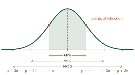
A bell-shaped Normal curve centred on mu. Vertical lines mark mu plus and minus sigma, 2 sigma and 3 sigma. Brackets show that about 68% of the area lies within one standard deviation of the mean, 95% within two and 99.7% within three. Dots mark the points of inflection at mu minus sigma and mu plus sigma — The same proportions hold for every Normal distribution. The curve changes from bending down to bending up at μ ± σ.

The shape of the Normal curve

Symmetric about $\mu$ , so the mean, median and mode are all $\mu$ .
About 68% of the distribution lies between $\mu - \sigma$ and $\mu + \sigma$ , 95% between $\mu - 2\sigma$ and $\mu + 2\sigma$ , and 99.7% between $\mu - 3\sigma$ and $\mu + 3\sigma$ .
Points of inflection at $x = \mu \pm \sigma$ .
The curve never touches the axis, but values more than $3\sigma$ from the mean are rare.

Why it works

The curve is $y = \dfrac{1}{\sigma\sqrt{2\pi}}\,e^{-\frac{1}{2}\left(\frac{x - \mu}{\sigma}\right)^2}$ . You won’t need to use it, but differentiating it twice, as in Chapter 13 of Year 2 Pure, shows that the second derivative is zero, and changes sign, exactly at $x = \mu \pm \sigma$ .

2. Finding probabilities

A probability for a Normal variable is the area under its curve, between two values or beyond one. There is no simple formula for these areas, so a calculator finds them.

On your calculator

The Normal cumulative distribution function takes a lower bound, an upper bound, $\sigma$ and $\mu$ , and returns the probability between them. For “less than $a$ ”, use a very large negative lower bound, such as $-10^{9}$ . The inverse Normal function goes the other way: from a probability to the value it lies below.

Worked example 3.1 · Apple masses

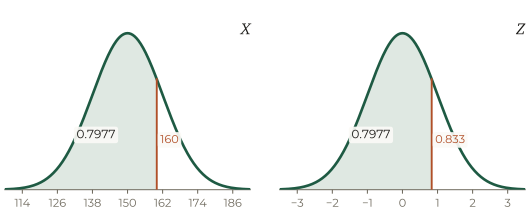
The masses of apples from an orchard are modelled by $X \sim N(150, 12^2)$ , in grams. Find the probability that an apple weighs less than $160$ g, and the probability that it weighs between $140$ g and $165$ g.

From the calculator, $P(X < 160) = 0.7977$ (4 d.p.).
$P(140 < X < 165) = 0.6920$ (4 d.p.).

In context

About 80% of apples weigh less than 160 g, and about 69% weigh between 140 g and 165 g.

Common mistake

The second parameter is the variance. $N(150, 12^2)$ has standard deviation $12$ , and the calculator wants $\sigma = 12$ , not $144$ . Read the question carefully: some write $N(150, 144)$ .

3. Standardising

Every Normal distribution is the same shape, stretched and shifted. Subtracting the mean and dividing by the standard deviation turns any of them into one standard curve.

The standard Normal distribution

If $X \sim N(\mu, \sigma^2)$ , then

Z = \frac{X - \mu}{\sigma}

has $Z \sim N(0, 1)$ . A value of $z$ says how many standard deviations $x$ lies above the mean. $P(Z < z)$ is written $\Phi(z)$ .

Two Normal curves side by side. The left is X distributed N of 150 and 12 squared with the area to the left of 160 shaded. The right is Z distributed N of 0 and 1 with the area to the left of 0.833 shaded. The shaded areas are equal, 0.7977 — 160 g is 10/12 = 0.833 standard deviations above the mean, so P(X < 160) = P(Z < 0.833).

Worked example 3.2 · The heaviest 10%

For the apples of Example 3.1, find the mass exceeded by only 10% of apples.

The inverse Normal gives $P(Z < 1.2816) = 0.9$ , so the mass is $1.2816$ standard deviations above the mean.
$m = 150 + 1.2816 \times 12 = 165.4$ g (1 d.p.). The calculator’s inverse Normal, with area $0.9$ , gives the same directly.

Standardising earns its keep when $\mu$ or $\sigma$ is unknown: the $z$ value comes from the probability, and the equation $x = \mu + z\sigma$ gives the missing parameter.

Worked example 3.3 · An unknown standard deviation

Times for a 100 m race are Normally distributed with mean $14.2$ s, and 20% of runners take less than $13.5$ s. Find the standard deviation.

$P(Z < z) = 0.2$ gives $z = -0.8416$ : $13.5$ s is $0.8416$ standard deviations below the mean.
So
$\begin{aligned} 13.5 &= 14.2 - 0.8416\sigma \\ \sigma &= 0.832 \text{ s (3 s.f.)} \end{aligned}$

Worked example 3.4 · Two unknowns

A random variable $X$ is Normally distributed. 10% of its values are more than $58$ , and 25% are less than $40$ . Find its mean and standard deviation.

$P(Z < z) = 0.9$ gives $z = 1.2816$ , and $P(Z < z) = 0.25$ gives $z = -0.6745$ . So
$\begin{aligned} \mu + 1.2816\sigma &= 58 \\ \mu - 0.6745\sigma &= 40 \end{aligned}$
Subtracting: $1.9561\sigma = 18$ , so $\sigma = 9.20$ (3 s.f.), and then $\mu = 58 - 1.2816 \times 9.202\ldots = 46.2$ (3 s.f.).

Common mistake

A value below the mean has a negative $z$ . If 20% lie below $13.5$ , then $13.5$ is below the mean, and $z = -0.8416$ , not $0.8416$ . A quick sketch with the area shaded catches the sign every time.

In the Normal view, set the mean and standard deviation and shade the area between two values: that area is the probability. The dots mark the points of inflection, one standard deviation either side of the mean. In the binomial view, the bars of B(n, p) sit under the Normal curve that approximates them, shaded with the continuity correction.

4. The Normal approximation to the binomial

A binomial histogram with large $n$ and $p$ near $0.5$ is almost exactly bell-shaped. The Normal curve with the same mean and variance then gives good approximations, with no long sums.

The Normal approximation

If $X \sim B(n, p)$ with $n$ large and $p$ close to $0.5$ , then $X$ is approximately $Y \sim N(np, np(1 - p))$ .

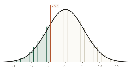
A binomial value $k$ covers the interval from $k - 0.5$ to $k + 0.5$ , so apply a continuity correction:

$P(X \le k) \approx P(Y < k + 0.5)$ ;
$P(X \ge k) \approx P(Y > k - 0.5)$ ;
$P(X = k) \approx P(k - 0.5 < Y < k + 0.5)$ .

A common guide is that the approximation is reasonable when both $np$ and $n(1 - p)$ are greater than $5$ .

A binomial bar chart for n = 80 and p = 0.4, with bars from 18 to 46. The Normal curve with mean 32 and variance 19.2 is drawn over it. The bars from 28 downwards are shaded, and the area under the curve to the left of 28.5 is shaded to match — Example 3.5: the bar for 28 runs from 27.5 to 28.5, so P(X ≤ 28) becomes P(Y < 28.5).

Worked example 3.5 · An approximation

$X \sim B(80, 0.4)$ . Use a Normal approximation to estimate $P(X \le 28)$ .

$np = 32$ and $np(1 - p) = 19.2$ , both large enough, so use $Y \sim N(32, 19.2)$ .
With a continuity correction, $P(X \le 28) \approx P(Y < 28.5) = 0.2122$ (4 d.p.).

In context

The exact binomial probability is $0.2131$ , so the approximation is out by less than $0.001$ .

5. Choosing a model

Is a Normal model sensible?

The variable is continuous, or discrete with many possible values.
The data are roughly symmetric and bell-shaped, with mean, median and mode close together.
About two-thirds of the data lie within one standard deviation of the mean, and almost all within three.
The model doesn’t give a noticeable probability to impossible values, such as negative lengths or times.

Practice

Twelve questions in three tiers. Try each one properly before opening the solution. The solutions show the full method, not just answers. Use a calculator’s Normal functions; give probabilities to 4 decimal places and other answers to 3 significant figures unless a question says otherwise.

Warm-up

1 [3 marks]

$X \sim N(20, 4^2)$ . Find (a) $P(X < 25)$ , (b) $P(X > 18)$ , (c) $P(16 < X < 22)$ .

Show solution

(a) $0.8944$ . (b) $0.6915$ . (c) $0.5328$ .

2 [3 marks]

$Z \sim N(0, 1)$ . Find $P(Z < 1.2)$ and $P(-0.5 < Z < 1.5)$ , and the value $z$ for which $P(Z > z) = 0.05$ .

Show solution

$P(Z < 1.2) = 0.8849$ and $P(-0.5 < Z < 1.5) = 0.6247$ .

$P(Z > z) = 0.05$ means $P(Z < z) = 0.95$ , so $z = 1.6449$ .

3 [2 marks]

$X \sim N(50, 10^2)$ . Find the value $a$ for which $P(X < a) = 0.3$ .

Show solution

$P(Z < z) = 0.3$ gives $z = -0.5244$ , so $a = 50 - 0.5244 \times 10 = 44.8$ .

4 [2 marks]

$X \sim N(70, 5^2)$ . Write down the $x$ -coordinates of the points of inflection of its curve, and an interval that contains about 95% of its values.

Show solution

The points of inflection are at $\mu \pm \sigma$ : $x = 65$ and $x = 75$ . About 95% of values lie within $2\sigma$ of the mean, between $60$ and $80$ .

Standard

5 [4 marks]

$X \sim N(100, \sigma^2)$ and $P(X > 110) = 0.15$ . Find $\sigma$ .

Show solution

$P(Z < z) = 0.85$ gives $z = 1.0364$ , so

\begin{aligned} 110 &= 100 + 1.0364\sigma \\ \sigma &= 9.65 \end{aligned}

6 [3 marks]

$X \sim N(\mu, 3^2)$ and $P(X < 20) = 0.8$ . Find $\mu$ .

Show solution

$P(Z < z) = 0.8$ gives $z = 0.8416$ , so $20 = \mu + 0.8416 \times 3$ and $\mu = 17.5$ .

7 [5 marks]

$X$ is Normally distributed, with $P(X < 30) = 0.2$ and $P(X > 60) = 0.1$ . Find its mean and standard deviation.

Show solution

$z = -0.8416$ for the lower 20%, and $z = 1.2816$ for the upper 10%:

\begin{aligned} \mu - 0.8416\sigma &= 30 \\ \mu + 1.2816\sigma &= 60 \end{aligned}

Subtracting: $2.1232\sigma = 30$ , so $\sigma = 14.1$ and $\mu = 30 + 0.8416 \times 14.12\ldots = 41.9$ .

8 [5 marks]

$X \sim B(50, 0.3)$ . Explain why a Normal approximation is reasonable, and use it to estimate $P(X \ge 20)$ .

Show solution

$np = 15$ and $n(1 - p) = 35$ are both greater than $5$ . Use $Y \sim N(15, 10.5)$ .

With a continuity correction, $P(X \ge 20) \approx P(Y > 19.5) = 0.0825$ .

9 [5 marks]

Adult heights in a town are modelled by $N(172, 7^2)$ , in cm.

Find the proportion of adults taller than 185 cm. [2]
Ten adults are chosen at random. Find the probability that at least one of them is taller than 185 cm. [3]

Show solution

(a) $P(H > 185) = 0.0316$ (4 d.p.).

(b) Each adult independently has probability $0.0316\ldots$ , so $P(\text{at least one}) = 1 - (1 - 0.0316\ldots)^{10} = 0.275$ (3 s.f.).

Exam style

10 [9 marks]

A machine fills bags of flour. Their masses are Normally distributed with mean $1005$ g, and 2% of bags weigh less than the stated $1000$ g.

Find the standard deviation of the masses. [3]
Find the probability that a bag weighs more than 1010 g. [2]
The machine’s mean is to be changed, with the standard deviation unchanged, so that only 0.5% of bags weigh less than 1000 g. Find the new mean. [4]

Show solution

(a) $P(Z < z) = 0.02$ gives $z = -2.0537$ , so $1000 = 1005 - 2.0537\sigma$ and $\sigma = 2.43$ g (3 s.f.).

(b) $1010$ g is as far above the mean as $1000$ g is below it, so by symmetry $P(M > 1010) = P(M < 1000) = 0.02$ .

(c) $P(Z < z) = 0.005$ gives $z = -2.5758$ , so $1000 = \mu - 2.5758 \times 2.434\ldots$ and $\mu = 1006$ g (4 s.f.).

11 [7 marks]

A multiple-choice test has 40 questions, each with five options. A student guesses every answer at random.

Using a Normal approximation, estimate the probability that the student scores at least 12. [5]
The exact binomial probability is 0.0875. Comment on the approximation. [2]

Show solution

(a) $X \sim B(40, 0.2)$ , with $np = 8$ and $np(1 - p) = 6.4$ . Use $Y \sim N(8, 6.4)$ , and correct for continuity:

P(X \ge 12) \approx P(Y > 11.5) = 0.0833

(b) It is a little low, out by about $0.004$ . $p = 0.2$ is far from $0.5$ , so the binomial distribution is skewed and the symmetric Normal curve fits it less well.

12 [6 marks]

The waiting times of 100 patients at a clinic have mean $6.2$ minutes and standard deviation $4.1$ minutes. The shortest wait was $0.5$ minutes and the longest $24$ minutes.

A manager models the waiting time by $N(6.2, 4.1^2)$ . Find the probability, according to the model, that a waiting time is negative. [2]
Give two reasons why the Normal model is not suitable. [4]

Show solution

(a) $P(W < 0) = 0.0652$ (4 d.p.).

(b) The model gives about 6.5% of patients a negative waiting time, which is impossible. And the longest wait, 24 minutes, is $\tfrac{24 - 6.2}{4.1} = 4.3$ standard deviations above the mean, which a Normal model makes almost impossible: the data are skewed, with a long tail of long waits.