Year 1 Statistics · Chapter 3

Representations of Data

Specification: Edexcel Paper 3 §2.1, 2.4 — Diagrams, outliers, cleaning data · AQA section L1, L4

Download chapter PDF Scroll this chapter

In this chapter

1. Histograms
2. Cumulative frequency
3. Box plots and outliers
4. Cleaning data
5. Comparing distributions
Practice

Key facts — this chapter

In a histogram, area represents frequency. With unequal classes the height is the frequency density $= \dfrac{\text{frequency}}{\text{class width}}$ .
A cumulative frequency curve plots the running total against the upper class boundary. Read the median at $\tfrac{n}{2}$ , the quartiles at $\tfrac{n}{4}$ and $\tfrac{3n}{4}$ .
A box plot shows five numbers: lowest value, $Q_1$ , median, $Q_3$ , highest value, with outliers marked separately.
The usual outlier rule: anything below $Q_1 - 1.5 \times \text{IQR}$ or above $Q_3 + 1.5 \times \text{IQR}$ . (Some questions use “more than 2 standard deviations from the mean” instead — always use the rule you are given.)
Cleaning data means dealing with errors, missing values and outliers. Only remove a value if there’s a reason to believe it’s wrong.
To compare distributions, compare location and spread, in context, and say which diagram supports each claim.

A summary statistic tells you one thing about a data set. A good diagram tells you the shape of the whole thing at a glance: where the values pile up, how far they spread, and whether anything odd is sitting out on its own.

1. Histograms

A histogram looks like a bar chart, but it means something different. Bar charts are for categories and the height carries the information. Histograms are for grouped continuous data, and the area carries it.

Area represents frequency

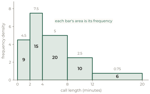
\text{frequency density} = \frac{\text{frequency}}{\text{class width}}

Plot frequency density on the vertical axis. Then each bar’s area is its frequency, and the bars touch (no gaps), because the classes run into each other.

Length, $t$ (min)	$0 \le t < 2$	$2 \le t < 4$	$4 \le t < 8$	$8 \le t < 12$	$12 \le t < 20$
Frequency	9	15	20	10	6
Class width	2	2	4	4	8
Frequency density	4.5	7.5	5	2.5	0.75

Lengths of 60 phone calls

A histogram of call lengths with unequal classes. Frequency densities are 4.5, 7.5, 5, 2.5 and 0.75, and each bar is labelled with its frequency: 9, 15, 20, 10 and 6 — The 4–8 class has 20 calls but a lower bar than 2–4, which has 15: it is twice as wide, so it spreads its frequency over twice the area.

Common mistake

Plotting the frequency as the height with unequal classes is the single most common error in this topic. It makes wide classes look far more common than they are. Check the wording too: “20 calls lasted between 4 and 8 minutes” is a frequency, while the bar’s height is the density.

Worked example 3.1 · Reading a histogram

In the histogram above, estimate the number of calls lasting between 5 and 8 minutes.

Those values lie in the class $4 \le t < 8$ , whose frequency density is 5. Assuming the calls are spread evenly through the class, use the area of that part of the bar:

\text{frequency} = \text{density} \times \text{width} = 5 \times (8 - 5) = 15\text{ calls}

When only a scale is given

Some questions give no vertical scale, just one bar’s frequency: “the bar for $2 \le t < 4$ has area 6 cm² and represents 15 calls”. Then every 6 cm² is 15 calls, so 1 cm² represents 2.5 calls, and you scale any other bar’s area the same way.

The same 60 phone calls, grouped in different ways. Click a bar to split it in two, or click a boundary mark (▲) to merge two classes. With frequency density on the vertical axis, every bar's area stays equal to its frequency, however you group the data.

classes

bar height

2. Cumulative frequency

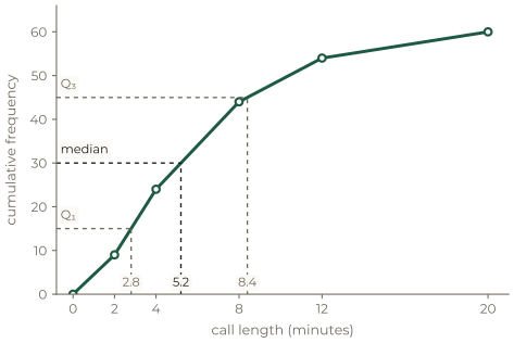
A cumulative frequency curve answers “how many are less than…?” Plot the running total against the upper class boundary of each class, and join the points with a smooth curve (or straight lines). Start at the lowest boundary with cumulative frequency 0.

A cumulative frequency curve for the call lengths, rising through (2, 9), (4, 24), (8, 44), (12, 54) and (20, 60), with dashed lines reading off the lower quartile 2.8, median 5.2 and upper quartile 8.4 — Read across at n/2 = 30 for the median, and at 15 and 45 for the quartiles.

Key result

From a cumulative frequency curve for $n$ values:

the median is read across from $\dfrac{n}{2}$ ;
$Q_1$ and $Q_3$ from $\dfrac{n}{4}$ and $\dfrac{3n}{4}$ ;
the $p$ th percentile from $\dfrac{pn}{100}$ .

Reading off the curve gives the same estimates as the interpolation in Chapter 2: the curve is the interpolation, drawn.

Worked example 3.2 · Using the curve

Use the curve to estimate the median call length, the interquartile range, and the number of calls lasting more than 10 minutes.

$n = 60$ , so read across at 30, 15 and 45:

Q_2 \approx 5.2, \qquad Q_1 \approx 2.8, \qquad Q_3 \approx 8.4

\text{IQR} \approx 8.4 - 2.8 = 5.6\text{ minutes}

At $t = 10$ the curve is at about 49, so about $60 - 49 = 11$ calls lasted more than 10 minutes.

3. Box plots and outliers

Outliers

A value is an outlier if it is

\text{below } Q_1 - 1.5 \times \text{IQR} \qquad\text{or}\qquad \text{above } Q_3 + 1.5 \times \text{IQR}

These two values are the fences. Some questions instead define an outlier as more than 2 (or 3) standard deviations from the mean. Use whichever rule the question gives.

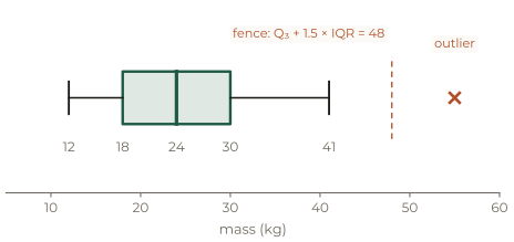
A box plot draws the five-number summary: lowest value, $Q_1$ , median, $Q_3$ , highest value. Any outliers are plotted as separate crosses, and the whisker then stops at the most extreme value that is not an outlier.

A box plot with lowest value 12, lower quartile 18, median 24, upper quartile 30 and whisker to 41, with an outlier marked with a cross at 55 and a dashed fence at 48 — IQR = 12, so the upper fence is 30 + 1.5 × 12 = 48. The value 55 lies beyond it, so it is plotted as an outlier and the whisker stops at 41.

Worked example 3.3 · Finding outliers

Fifteen parcels have masses, in kg: 12, 15, 17, 18, 20, 21, 22, 24, 25, 26, 28, 30, 33, 41, 55. Show that 55 kg is an outlier and 41 kg is not, then describe the box plot.

With $n = 15$ : $\dfrac{n}{4} = 3.75$ , so $Q_1$ is the 4th value, 18. The median is the 8th value, 24. $\dfrac{3n}{4} = 11.25$ , so $Q_3$ is the 12th value, 30.

\text{IQR} = 30 - 18 = 12, \qquad Q_1 - 1.5(12) = 0, \qquad Q_3 + 1.5(12) = 48

$55 > 48$ , so 55 kg is an outlier. $41 < 48$ , so 41 kg is not.

In context

The box runs from 18 to 30 with the median at 24. The left whisker reaches the lowest value, 12; the right whisker stops at 41, the largest value inside the fence; and 55 is plotted as a cross.

4. Cleaning data

Real data contain mistakes. Cleaning means deciding what to do with values that look wrong before any analysis.

Key result

An error (a height of 17 m, a negative age) can be removed or corrected.
A missing value is usually left out, and you say so.
A genuine outlier is not automatically wrong. Only remove a value if you have a reason: a recording error, or a unit mix-up. Otherwise keep it and mention it.

Common mistake

“Remove the outlier because it is far from the others” is circular, and earns no marks. Give a reason it’s likely to be invalid — “a call of 0 minutes was probably a misdial” — or keep the value and comment on its effect.

5. Comparing distributions

Key result

Compare location and spread, in context, and say which feature of the diagram you’re using:

box plots: compare medians and IQRs, and mention skew or outliers;
histograms: compare shape, where the bulk of the data sits, and any tail;
cumulative frequency curves: compare medians, quartiles and how steeply each curve rises.

In context

“The median mass for the parcels from depot B (30 kg) is higher than for depot A (24 kg), so B’s parcels are typically heavier. B’s IQR (11 kg) is a little smaller than A’s (12 kg), so its masses are slightly more consistent. A also has an outlier at 55 kg, which B does not.”

Practice

Twelve questions in three tiers. Try each one properly before opening the solution. Unless a question says otherwise, treat a value as an outlier if it is more than $1.5 \times \text{IQR}$ beyond a quartile.

Warm-up

1 [3 marks]

Find the frequency density of each class.

Class	$0 \le x < 5$	$5 \le x < 15$	$15 \le x < 20$	$20 \le x < 40$
Frequency	8	25	12	10

Show solution

Divide each frequency by its class width (5, 10, 5, 20):

Class	$0 \le x < 5$	$5 \le x < 15$	$15 \le x < 20$	$20 \le x < 40$
Frequency density	1.6	2.5	2.4	0.5

2 [3 marks]

In a histogram, the bar for the class $10 \le x < 20$ has height 3.2.

Find the frequency of that class.
The class $20 \le x < 25$ has frequency 18. Find the height of its bar.

Show solution

(a) Frequency $= \text{density} \times \text{width} = 3.2 \times 10 = 32$ .

(b) Density $= \dfrac{18}{5} = 3.6$ .

3 [3 marks]

The distances travelled to work by 50 commuters are grouped below.

Distance, $d$ (km)	$0 \le d < 5$	$5 \le d < 10$	$10 \le d < 20$	$20 \le d < 30$	$30 \le d < 50$
Frequency	7	13	18	8	4

Write down the cumulative frequencies.
State how many commuters travel less than 20 km.

Show solution

(a) 7, 20, 38, 46, 50, plotted against the upper boundaries 5, 10, 20, 30, 50.

(b) 38 commuters.

4 [4 marks]

Eleven values, in order, are 4, 6, 7, 9, 11, 12, 14, 15, 18, 21, 30.

Find the quartiles and the IQR.
Determine whether 30 is an outlier.

Show solution

(a) $\dfrac{n}{4} = 2.75$ , so $Q_1$ is the 3rd value, 7. The median is the 6th value, 12. $\dfrac{3n}{4} = 8.25$ , so $Q_3$ is the 9th value, 18. $\text{IQR} = 18 - 7 = 11$ .

(b) The fences are $7 - 1.5(11) = -9.5$ and $18 + 1.5(11) = 34.5$ . Since $30 < 34.5$ , the value 30 is not an outlier, even though it looks far from the rest.

Standard

5 [4 marks]

In a histogram, the bar for $0 \le x < 10$ has area $4.8\text{ cm}^2$ and represents 24 values.

Find how many values $1\text{ cm}^2$ represents.
Another bar has area $3.2\text{ cm}^2$ . Find its frequency.

Show solution

(a) $\dfrac{24}{4.8} = 5$ values per $\text{cm}^2$ .

(b) $3.2 \times 5 = 16$ values.

6 [6 marks]

The heights, $h$ cm, of 80 plants are grouped below.

Height, $h$ (cm)	$100 \le h < 120$	$120 \le h < 130$	$130 \le h < 140$	$140 \le h < 160$	$160 \le h < 200$
Frequency	12	18	24	16	10

Heights of 80 plants

Find the frequency density of each class.
Estimate the number of plants between 125 cm and 135 cm tall.

Show solution

(a) 0.6, 1.8, 2.4, 0.8 and 0.25.

(b) Half of the class $120 \le h < 130$ and half of $130 \le h < 140$ , using areas:

1.8 \times 5 + 2.4 \times 5 = 9 + 12 = 21\text{ plants}

7 [7 marks]

The times, $t$ minutes, of 80 runners in a race are grouped below.

Time, $t$ (min)	$20 \le t < 25$	$25 \le t < 30$	$30 \le t < 35$	$35 \le t < 40$	$40 \le t < 50$	$50 \le t < 60$
Frequency	6	14	22	20	14	4

Race times of 80 runners

Write down the cumulative frequencies.
Estimate the median and the interquartile range.
Estimate how many runners took longer than 45 minutes.

Show solution

(a) 6, 20, 42, 62, 76, 80.

(b) $k = 40$ , in $30 \le t < 35$ : $Q_2 \approx 30 + \dfrac{40 - 20}{22} \times 5 = 34.5$ min (3 s.f.).

$k = 20$ is exactly the cumulative frequency at 30, so $Q_1 \approx 30$ min. $k = 60$ , in $35 \le t < 40$ : $Q_3 \approx 35 + \dfrac{60 - 42}{20} \times 5 = 39.5$ min.

$\text{IQR} \approx 39.5 - 30 = 9.5$ min.

(c) Half of the class $40 \le t < 50$ lies above 45, so the cumulative frequency at 45 is about $62 + 7 = 69$ . That leaves about $80 - 69 = 11$ runners.

8 [4 marks]

For a set of test marks the mean is 52 and the standard deviation is 6. A mark is defined as an outlier if it is more than two standard deviations from the mean.

Find the range of marks that are not outliers.
State whether the marks 39, 41 and 65 are outliers.

Show solution

(a) $52 \pm 2(6)$ , so marks from 40 to 64 are not outliers.

(b) 39 is an outlier, since it is below 40. 41 is not, since it lies inside the range. 65 is an outlier, since it is above 64.

Exam style

9 [8 marks]

The masses, $m$ grams, of 120 apples are shown in a histogram. The frequency densities are given below.

Mass, $m$ (g)	$60 \le m < 80$	$80 \le m < 90$	$90 \le m < 100$	$100 \le m < 120$	$120 \le m < 160$
Frequency density	0.9	2.4	3.6	1.2	?

Masses of 120 apples

Find the frequency of each of the first four classes.
Hence find the missing frequency density.
Estimate the median mass.
Estimate the percentage of apples with mass over 110 g.

Show solution

(a) Multiply density by width: $0.9 \times 20 = 18$ , $2.4 \times 10 = 24$ , $3.6 \times 10 = 36$ , $1.2 \times 20 = 24$ .

(b) Those account for $18 + 24 + 36 + 24 = 102$ apples, so the last class has $120 - 102 = 18$ , and its density is $\dfrac{18}{40} = 0.45$ .

(c) $k = 60$ . The cumulative frequencies are 18, 42, 78, so the median is in $90 \le m < 100$ :

Q_2 \approx 90 + \frac{60 - 42}{36} \times 10 = 95\text{ g}

(d) Above 110 g: half of $100 \le m < 120$ , which is 12 apples, plus all 18 in the last class, giving 30.

\frac{30}{120} = 25\%

10 [6 marks]

Depot A’s parcels have the five-number summary 12, 18, 24, 30, 41 kg, with one outlier at 55 kg. Depot B’s 15 parcels are, in kg: 20, 22, 23, 25, 26, 27, 29, 30, 31, 33, 35, 36, 38, 40, 44.

Find the quartiles for depot B and show that it has no outliers.
Compare the two depots’ parcel masses.

Show solution

(a) $\dfrac{n}{4} = 3.75$ , so $Q_1$ is the 4th value, 25. The median is the 8th, 30. $\dfrac{3n}{4} = 11.25$ , so $Q_3$ is the 12th, 36. $\text{IQR} = 11$ .

Fences: $25 - 1.5(11) = 8.5$ and $36 + 1.5(11) = 52.5$ . The smallest value (20) and the largest (44) both lie inside, so there are no outliers.

(b) B’s median (30 kg) is higher than A’s (24 kg), so B’s parcels are typically heavier. B’s IQR (11 kg) is slightly smaller than A’s (12 kg), so B’s masses are a little more consistent. A also has an outlier at 55 kg, far heavier than anything from B.

11 [6 marks]

A student records the reaction times, in seconds, of 12 people. One person’s time was not recorded. The others are:

0.28, 0.31, 0.33, 0.29, 3.2, 0.35, 0.30, 0.27, 0.32, 0.34, 0.31

Calculate the mean of the 11 recorded times.
Explain why the value 3.2 should be investigated, and suggest what went wrong.
The student decides the 3.2 should have been 0.32. Recalculate the mean and comment.

Show solution

(a) The total is 6.30, so the mean is $\dfrac{6.30}{11} = 0.573$ s (3 s.f.).

(b) Every other time is around 0.3 s, so 3.2 s is roughly ten times larger than the rest. Human reaction times are not that slow, so it is almost certainly a recording error: most likely a misplaced decimal point (0.32 typed as 3.2).

(c) The corrected total is 3.42, so the mean is $\dfrac{3.42}{11} = 0.311$ s (3 s.f.).

In context

One mistyped value pushed the mean from 0.311 s to 0.573 s — nearly double — even though every other reading was fine. That’s why data are cleaned before they are summarised. The missing 12th value is simply left out, and the report should say the mean is based on 11 times.

12 [7 marks]

A cumulative frequency curve for the lengths of 60 phone calls gives $Q_1 = 2.8$ , $Q_2 = 5.2$ and $Q_3 = 8.4$ minutes. The shortest call was 0.4 minutes and the longest was 19 minutes.

Show that any call longer than 16.8 minutes is an outlier.
Describe the box plot for these data.
The curve shows 6 calls in the class $12 \le t < 20$ . Explain why you cannot tell from the curve exactly how many calls are outliers.

Show solution

(a) $\text{IQR} = 8.4 - 2.8 = 5.6$ , so the upper fence is

Q_3 + 1.5 \times \text{IQR} = 8.4 + 8.4 = 16.8\text{ minutes}

Any call longer than this is an outlier. (The lower fence is $2.8 - 8.4 = -5.6$ , so no short call can be an outlier.)

(b) A box from 2.8 to 8.4 with the median at 5.2. The left whisker runs to 0.4. The longest call, 19 minutes, is beyond the fence, so it is plotted as an outlier, and the right whisker stops at the largest call of 16.8 minutes or less.

(c) The curve only gives the number of calls in each class, not the individual values. The 6 calls between 12 and 20 minutes could all be under 16.8, or several could be above it. You would need the raw data to count the outliers exactly.