Year 1 Statistics · Chapter 2
Measures of Location and Spread
Specification: Edexcel Paper 3 §2.3 — Measures of central tendency and variation · AQA section L3
In this chapter
Key facts — this chapter
- Mean , or from a frequency table. The median is the middle value; the mode is the most common.
- Quartiles split ordered data into four equal parts. IQR is the spread of the middle half.
- For grouped data, estimate the mean with class midpoints, and estimate the median, quartiles and percentiles by linear interpolation.
- Variance . The standard deviation is its square root: the typical distance from the mean.
- Coding : then and . Adding or subtracting moves the mean but not the spread.
- When comparing data sets, compare a measure of location and a measure of spread, in context.
Two numbers summarise most data sets: one for where the values sit (location) and one for how widely they spread. This chapter builds the standard choices for each, shows how to get them from raw data, frequency tables and grouped data, and ends with the skill examiners reward most: saying what they mean.
1. Averages
Key result
The median is the middle value of the ordered data. The mode is the most frequent value (or the modal class for grouped data).
Each average has its strengths:
| Average | Use it when… | Watch out for… |
|---|---|---|
| mean | you want every value to count; no extreme values | it is pulled towards outliers |
| median | there are outliers or the data are skewed | it ignores the size of extreme values |
| mode | the data are qualitative, or you want the most common value | there may be no mode, or several |
For grouped data you don’t know the exact values, so each class is represented by its midpoint and the mean is an estimate.
2. Quartiles, percentiles and the IQR
The lower quartile , median and upper quartile cut the ordered data into four equal parts. The interquartile range measures the spread of the middle 50%, so it ignores the extremes at both ends. Percentiles divide the data into 100 parts, and the 10th to 90th percentile range is another spread measure that is robust to extremes.
Quartiles of raw (discrete) data
For ordered values, to find work out :
- if it is not a whole number, round up and take that value;
- if it is a whole number, take the mean of that value and the next one.
Use for the median and for in the same way.
Worked example 2.1 · Averages and quartiles from raw data
The times, in minutes, that 11 people took to complete a puzzle were 12, 15, 9, 22, 17, 15, 11, 19, 14, 15, 20. Find the mean, median, mode, quartiles and interquartile range.
In order: 9, 11, 12, 14, 15, 15, 15, 17, 19, 20, 22.
- Mean: minutes (3 s.f.). Mode: 15 minutes.
- , so round up: the median is the 6th value, 15 minutes.
- , so is the 3rd value, 12. , so is the 9th value, 19.
- minutes.
Grouped data: linear interpolation
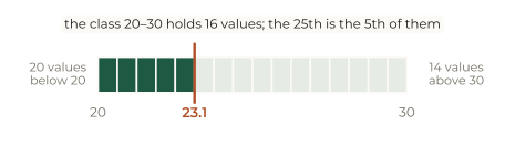
In grouped continuous data the values inside a class are unknown, so assume they are spread evenly through it. Then a value’s position within its class gives its size.
Linear interpolation
To estimate the value at position (use for the median, for , for , for the th percentile):
where is the lower boundary of the class containing position , is the cumulative frequency before that class, is its frequency and is its width. (Named in Edexcel’s guidance, and the standard method for both boards.)
Worked example 2.2 · Estimates from grouped data
The table shows the journey times of 50 students. Estimate the mean, the median, the quartiles and the 90th percentile.
| Time, (minutes) | |||||
|---|---|---|---|---|---|
| Frequency, | 6 | 14 | 16 | 10 | 4 |
| Midpoint, | 5 | 15 | 25 | 35 | 50 |
| Cumulative frequency | 6 | 20 | 36 | 46 | 50 |
Mean: , so minutes.
Median: , which lies in (20 values come before it):
Quartiles: () and () , so the IQR is about 16.9 minutes.
90th percentile: , in : minutes.
Common mistake
For grouped continuous data use , not , and don’t round positions: interpolation handles fractions. The “round up” rule is only for raw discrete data.
3. Variance and standard deviation
The IQR ignores most of the data. The standard deviation uses every value: it measures how far, typically, the values sit from the mean.
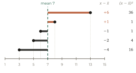
Variance and standard deviation
From a frequency table: .
The second form of the variance, “the mean of the squares minus the square of the mean”, is the one to calculate with. It only needs , and , which questions often give you instead of the raw data (the summary statistics).
Worked example 2.3 · From summary statistics
For 20 values, and . Find the mean and the standard deviation.
Worked example 2.4 · From a frequency table
The numbers of goals scored in 30 matches are shown below. Find the mean, median and standard deviation.
| Goals, | 0 | 1 | 2 | 3 | 4 | 5 |
|---|---|---|---|---|---|---|
| Frequency, | 4 | 8 | 9 | 5 | 3 | 1 |
, and .
goals (3 s.f.).
The median is the mean of the 15th and 16th values. The cumulative frequencies are 4, 12, 21, …, so both are 2: the median is 2 goals.
On your calculator
The 1-variable statistics mode gives , , and two standard deviations. divides by , as in this chapter. divides by : AQA accepts either, but Edexcel expects . Enter frequency tables with the frequency column switched on.
Drag the dots to change the data. The mean, median, quartiles and standard deviation update as you go. Then code every value at once and watch which measures move.
4. Coding
Awkward numbers can be coded to simpler ones, for example . Work with , then decode. (Named in Edexcel’s guidance.)
Coding
If , then
Subtracting shifts every value, and so the mean, but leaves the spread alone. Dividing by scales both.
Worked example 2.5 · Decoding
Heights cm were coded using , giving and . Find the mean and standard deviation of the heights.
Rearrange: . So cm and cm. The affects the mean only.
5. Comparing distributions
Key result
To compare two data sets, make two comparisons, each in context:
- a measure of location: mean or median;
- a measure of spread: standard deviation, IQR or range.
Pair them sensibly: mean with standard deviation, or median with IQR (the median and IQR are better if there are outliers).
In context
“The mean time for Class A (15.4 min) was lower than for Class B (18.1 min), so on average Class A completed the puzzle faster. Class A’s standard deviation (3.75 min) was also smaller than Class B’s (6.2 min), so their times were more consistent.”
Common mistake
“Class A has a lower mean” earns nothing on its own. Say what it means for the people or things in the question: “on average, Class A were faster”. The context sentence carries the marks.
Practice
Twelve questions in three tiers. Try each one properly before opening the solution. Give answers to 3 significant figures where they are not exact, and use the divisor for variance and standard deviation.
Warm-up
Ten students scored: 13, 7, 21, 4, 10, 15, 7, 18, 8, 12.
Find the mean, the median and the mode.
Show solution
Mean .
In order: 4, 7, 7, 8, 10, 12, 13, 15, 18, 21. Here , a whole number, so the median is the mean of the 5th and 6th values: .
Mode .
Twelve values, in order, are 3, 5, 6, 8, 9, 11, 12, 14, 15, 17, 20, 24. Find the median, the quartiles and the interquartile range.
Show solution
, so .
, so .
, so .
.
The table shows the number of pets owned by 25 students.
| Pets, | 0 | 1 | 2 | 3 |
|---|---|---|---|---|
| Frequency, | 7 | 10 | 6 | 2 |
Find the mean, the median and the mode.
Show solution
, so the mean is pets.
, so round up: the median is the 13th value. The cumulative frequencies are 7, 17, …, so the 13th value is 1 pet.
The mode is 1 pet (the highest frequency, 10).
Find the mean and standard deviation of 2, 4, 4, 4, 5, 5, 7, 9.
Show solution
, so .
, so
Standard
For a set of 15 values, and .
- Find the mean and the standard deviation.
- A 16th value, 18, is added to the set. Find the new mean and standard deviation.
- Explain why the standard deviation changed as it did.
Show solution
(a) and , so (3 s.f.).
(b) Now , and .
and , so (3 s.f.).
(c) The new value equals the mean, so the mean is unchanged, but it adds a deviation of zero to the set. The average squared deviation therefore falls, and the standard deviation with it.
The heights, cm, of 40 seedlings are shown below.
| Height, (cm) | |||||
|---|---|---|---|---|---|
| Frequency | 4 | 10 | 15 | 8 | 3 |
- Write down the modal class.
- Estimate the mean height.
- Estimate the median height.
Show solution
(a) (frequency 15).
(b) Midpoints 2.5, 7.5, 12.5, 17.5, 25:
(c) . The cumulative frequencies are 4, 14, 29, so the median is in :
The values were coded using . For the 10 coded values, and .
- Find the mean and standard deviation of .
- Hence find the mean and standard deviation of .
Show solution
(a) and , so (3 s.f.).
(b) , so and (3 s.f.).
Using the seedling data from Question 6:
- Estimate the lower and upper quartiles, and the interquartile range.
- Estimate the 90th percentile.
Show solution
Cumulative frequencies: 4, 14, 29, 37, 40.
(a) : , in , so cm.
: , in , so cm (3 s.f.).
cm (3 s.f.).
(b) , in : cm (3 s.f.).
Exam style
Two classes sat the same test. Class A had mean 62 marks, standard deviation 8.5, median 64 and IQR 10. Class B had mean 58 marks, standard deviation 14, median 62 and IQR 21.
- Compare the two classes’ results.
- Class B’s teacher says the class contains a few very low marks. Explain how the given statistics support this, and say which pair of measures is the better summary for Class B.
Show solution
(a) Class A’s mean (62) is higher than Class B’s (58), so on average Class A did better on the test. Class A’s standard deviation (8.5) is much smaller than Class B’s (14), so Class A’s marks were far more consistent, while Class B’s were widely spread.
(b) For Class B the mean (58) is below the median (62). A few very low marks drag the mean down while barely moving the median, which is exactly the pattern here, and they also inflate the standard deviation (14) and the IQR (21). Since extreme values distort the mean and standard deviation, the median and IQR are the better summary for Class B.
The waiting times, minutes, of 80 patients at a clinic are recorded.
| Time, (min) | |||||
|---|---|---|---|---|---|
| Frequency | 12 | 25 | 20 | 15 | 8 |
- Estimate the mean and the standard deviation.
- Estimate the median.
- Explain why your answers are estimates.
Show solution
(a) Midpoints 2.5, 7.5, 12.5, 20, 32.5.
, so min (3 s.f.).
, so
(b) . Cumulative frequencies are 12, 37, 57, so the median lies in :
(c) The original values are lost once the data are grouped. The calculations assume every value sits at its class midpoint (for the mean) or that values are evenly spread through the class (for the median), and neither is exactly true.
Group 1 has 12 values with mean 15 and standard deviation 2. Group 2 has 8 values with mean 20 and standard deviation 3. Find the mean and standard deviation of all 20 values combined.
Show solution
Mean: , so .
Sums of squares: from we get :
In context
The combined standard deviation (3.46) is bigger than either group’s, because the two groups are centred on different means: that gap adds to the overall spread.
For 25 values a student calculates a mean of 40 and a standard deviation of 6. She then notices that one value was recorded as 52 when it should have been 42.
- Find the correct mean.
- Find the correct standard deviation.
Show solution
(a) From the wrong data, . Correcting the value: , so the mean is .
(b) From . Correcting:
In context
Correcting one value that was too high pulls both the mean and the spread down.