Year 1 Statistics · Chapter 4
Correlation
Specification: Edexcel Paper 3 §2.2 — Bivariate data · AQA section L2
In this chapter
Key facts — this chapter
- Bivariate data pair two measurements for each item. Plot them on a scatter diagram, with the explanatory variable on the -axis and the response variable on the -axis.
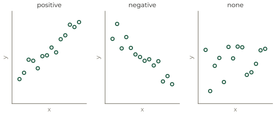
- Correlation describes a linear pattern: positive (as one rises, so does the other), negative (one rises as the other falls), or none.
- A regression line is the line of best fit. In Year 1 it is always given to you. The gradient is the change in per unit of ; the intercept is the value of when .
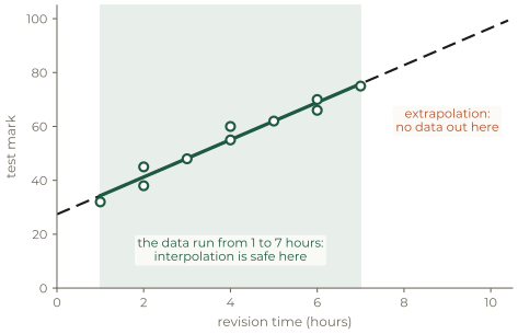
- Predicting inside the range of the data is interpolation (reasonably reliable); predicting outside it is extrapolation (unreliable, because you have no evidence the pattern continues).
- Correlation does not imply causation. A third variable may explain both, or the link may be coincidence.
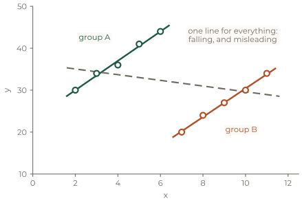
- Watch for distinct subgroups: a single line through two different groups can point the opposite way to each group.
So far each chapter has handled one variable at a time. Bivariate data come in pairs — a temperature and a sales figure, hours of revision and a mark — and the question becomes whether the two move together, and what you can safely predict from that.
1. Scatter diagrams and correlation
Plot each pair as a point. By convention the explanatory (independent) variable goes on the horizontal axis, and the response (dependent) variable, the one you think is being affected, on the vertical axis.
Key result
Describe correlation with two words: its direction (positive or negative) and its strength (strong, moderate, weak) — then say what it means in context.
In context
“The scatter shows strong positive correlation: students who revised for longer generally scored higher marks.”
Common mistake
“There is a correlation” on its own earns nothing. Name the direction, and describe it in the words of the question. And correlation is about a linear pattern: a clear curved relationship can have almost no linear correlation at all.
2. The regression line
The regression line of on is the straight line that best fits the data, chosen to make the vertical gaps between the points and the line as small as possible. You will always be given its equation — calculating it is Year 2 work.
Interpreting y = a + bx
- (the gradient) is the change in for each 1 unit increase in .
- (the intercept) is the value of predicted when . It’s only meaningful if is near or inside the data.
Always interpret both with units, in context.
Worked example 4.1 · Using a given line
For ten students, the regression line of test mark on revision time hours is . The revision times in the sample ranged from 1 to 7 hours.
(a) Interpret the gradient. (b) Predict the mark of a student who revises for 3.5 hours. (c) Predict the mark for 10 hours and comment.
(a) Each extra hour of revision is associated with about 6.9 more marks.
(b) , so about 52 marks. This is interpolation — 3.5 hours is inside the range 1 to 7 — so it should be reasonably reliable.
(c) , so about 97 marks. But 10 hours is well outside the data, so this is extrapolation and unreliable: the improvement may level off with tiredness, and the model would happily predict over 100 marks for 11 hours.
In context
Use the line for students revising between 1 and 7 hours, and treat anything outside that range with caution.
Common mistake
The intercept is often nonsense in context. Here claims a student who revises for 0 hours scores 27 marks — but nobody in the sample revised for less than an hour, so that’s extrapolation too. Say so when you interpret it.
Drag any point to change the data. The line of best fit follows, and the shaded band shows the range the data actually cover. Move the prediction marker outside that band and the reading turns into a guess.
3. Correlation and causation
A strong correlation does not mean one variable causes the other. There are three explanations to weigh every time.
Key result
- One variable really does affect the other.
- A third variable affects both. (Ice cream sales and sunburn cases rise together, but the weather drives both.)
- Coincidence, particularly in small samples.
Only a controlled experiment, not a scatter diagram, can establish cause.
Worked example 4.2 · Judging a claim
A newspaper reports strong positive correlation between the number of hours children spend on homework and their height, and concludes that homework makes children taller. Comment.
The conclusion doesn’t follow. Age explains both: older children are taller and are set more homework. Age is a third variable driving the two together, so the correlation is real but the causal claim is not.
4. Subgroups in one scatter
If a data set mixes two different groups, a single line can be badly misleading.
Why the line flips
Group B sits to the right of group A but lower down. Fitting one line to the combined data mostly measures the gap between the groups, not the pattern inside them. It’s a reminder that a regression line summarises whatever you feed it, sensibly or not.
In context
“The scatter shows two distinct groups. Within each group the correlation is positive, so a single regression line for all the data would be misleading. It would be better to fit a separate line to each group.”
Practice
Twelve questions in three tiers. Try each one properly before opening the solution. In this chapter every regression line is given: the marks are for using and criticising it, in context.
Warm-up
For each pair of variables, state the correlation you would expect and which variable you would plot on the -axis.
- The age of a car and its value.
- A person’s height and their shoe size.
- A person’s house number and their exam mark.
Show solution
(a) Negative correlation: older cars are worth less. Age is the explanatory variable, so it goes on the -axis.
(b) Positive correlation: taller people tend to have larger feet. Height on the -axis.
(c) No correlation: the two are unrelated. (Either could go on the -axis, since neither explains the other.)
The regression line of on is .
- Predict when .
- Interpret the gradient.
Show solution
(a) .
(b) For each increase of 1 in , increases by about 3.4.
A regression line is based on data with values from 2 to 15. State whether using the line to predict at each of these values is interpolation or extrapolation, and which prediction you would trust.
Show solution
(a) Interpolation, since 5 lies inside the range 2 to 15. This prediction can be trusted (as far as the model fits).
(b) Extrapolation, since 20 is outside the range. There is no evidence the pattern continues that far, so it is unreliable.
In a seaside town, weekly ice cream sales and the number of people treated for sunburn show strong positive correlation. A student concludes that eating ice cream causes sunburn. Explain why this conclusion is wrong.
Show solution
Correlation does not imply causation. A third variable — hot, sunny weather — increases both ice cream sales and the time people spend outside getting sunburnt. The two rise together without either causing the other.
Standard
For ten days, a café records the midday temperature °C and the number of cold drinks sold, . The temperatures ranged from 12 °C to 26 °C, and the regression line is .
- Interpret the gradient in context.
- Estimate the sales when the temperature is 19 °C.
- Estimate the sales at 35 °C and comment on your answer.
Show solution
(a) For each 1 °C rise in midday temperature, the café sells about 4.9 more cold drinks.
(b) , so about 119 drinks. This is interpolation, so it should be reasonably reliable.
(c) , so about 197 drinks. But 35 °C is far outside the recorded range of 12–26 °C, so this is extrapolation. Sales might level off once the café runs out of stock or seats, so the estimate is unreliable.
The regression line of a car’s value (£) on its age years is , based on cars aged 1 to 9 years.
- Interpret the gradient and the intercept in context.
- Explain why the model cannot be used for a 12-year-old car.
Show solution
(a) The value falls by about £1750 for each extra year of age. The intercept suggests a new car (age 0) would be worth £14 500, though no car in the sample was new, so that is an extrapolation.
(b) 12 years is outside the range 1 to 9 years. The model would predict , a negative value, which is impossible: the linear pattern clearly does not continue.
A scatter diagram of against shows two clearly separated clusters of points. Within each cluster the points rise from left to right, but a single regression line fitted to all the data has a negative gradient.
- Explain how this can happen.
- State what should be done instead.
Show solution
(a) The second cluster lies to the right of the first but lower down. A single line mostly measures the difference between the two groups rather than the pattern within them, so it slopes the opposite way.
(b) The data should be separated, with a regression line fitted to each group, and the two groups described separately. The scatter should always be looked at, not just the equation of the line.
The table shows the mass, kg, and the length, cm, of eight fish.
| Length, (cm) | 18 | 22 | 25 | 27 | 30 | 33 | 36 | 40 |
|---|---|---|---|---|---|---|---|---|
| Mass, (kg) | 0.9 | 1.3 | 1.6 | 1.9 | 2.4 | 2.8 | 3.3 | 4.1 |
- Describe the correlation and what it means here.
- Which variable is the explanatory variable? Justify your choice.
- A ninth fish is 24 cm long with mass 3.9 kg. Describe where it would lie on the scatter, and what you would do about it.
Show solution
(a) Strong positive correlation: longer fish tend to be heavier.
(b) Length. A fish’s mass depends on its size, rather than the other way round, so length goes on the -axis as the explanatory variable.
(c) It would sit well above the pattern: at 24 cm the other fish weigh around 1.5 kg, so 3.9 kg is far heavier than expected. It should be investigated as a possible recording error before being included. If it is genuine, it should be kept and commented on, since it may be a different species.
Exam style
Ten students’ weekly study hours and end-of-term scores are recorded. The study times range from 5 to 28 hours, and the regression line is .
- Interpret the gradient in context.
- Estimate the score of a student who studies 14 hours a week.
- Estimate the score for 40 hours a week, and give two reasons to distrust it.
- A student says the line proves that studying causes higher scores. Comment.
Show solution
(a) Each extra hour of study per week is associated with about 1.06 more marks.
(b) , so about 52 marks (interpolation, so reasonably reliable).
(c) , so about 80 marks. Two reasons to distrust it: 40 hours is far outside the range 5–28 hours (extrapolation), and the relationship is unlikely to stay linear — extra hours probably have less and less effect, and tiredness may reduce performance.
(d) The data show association, not cause. More able or better-motivated students may both study more and score higher, so a third factor could explain the link. Only a controlled experiment could establish cause.
A study finds that towns with more libraries per person have higher average exam results, and recommends building more libraries to raise results.
- Give a possible third variable that could explain the correlation.
- Explain the danger of acting on this recommendation.
- Describe what evidence would be needed to support the claim.
Show solution
(a) The wealth of the town. Wealthier areas can fund more libraries and tend to have better-resourced schools, which raises results.
(b) If wealth is the real driver, building libraries alone may not improve results at all, and the money might be better spent directly on schools.
(c) A controlled study: compare similar towns where libraries are added with ones where they are not, over time, keeping other factors as alike as possible.
The regression line of on for some data is . A student wants to estimate the value of when , so writes and gets .
- Explain why this is not the recommended way to estimate from .
- State the circumstances in which the estimate would still be reasonable.
Show solution
(a) The regression line of on is chosen to make the vertical distances from the points small, so it is designed for predicting from . Rearranging it to predict from is not the same as the line of on , which would be fitted the other way round, and it generally gives a different answer.
(b) If the correlation is very strong, the two lines are close together, so the estimate is reasonable — provided also lies inside the range of the observed values.
A biologist measures the height of a plant each week for 12 weeks. The regression line of height cm on week is , and the scatter shows the points lying close to a straight line for the first 8 weeks, then curving and flattening out.
- Comment on the suitability of a linear model for these data.
- The biologist predicts the height in week 20. Give two criticisms of this prediction.
- Suggest how the model could be improved.
Show solution
(a) A straight line fits the first 8 weeks well, but the later points curve away from it. Over the whole 12 weeks, a linear model is not suitable: it will overestimate the later heights.
(b) Week 20 is outside the data (extrapolation), and the pattern was already bending away from the line by week 12, so the linear trend has clearly stopped. The prediction of cm is almost certainly far too high.
(c) Use a model that levels off, since plants approach a maximum height — for example fitting a curve, or a straight line only to the first 8 weeks while stating that it applies to that period alone.